The Golden Ratio Discharge a fundamental part of The Wheelwork of Nature, revealing the underlying natural order expressed within electricity. (Click to enlarge images, and hover to pause slides)
The Golden Ratio Discharge showing well defined order, symmetry, as well as spatial and temporal coherence and choreography.
The Golden Ratio Discharge, also known as The Fractal-Fern Discharge, has its best fit in the form of The Golden Dragon, which is a fractal that expands according to the Golden Ratio.
The AMInnovations MiniGen is a complete portable vacuum tube Tesla coil generator, and suitable for a wide range of different electricity experiments and demonstrations.
High-Efficency Transference of Electric Power experiments passing 500W of power across a 40awg (80 micron) single wire at an efficiency over 99.5%.
Plasma discharge, induction, and tension experiments using specialised Tesla Transformers driven by a vacuum tube generator, and similar in design to Eric Dollard's cosmic induction generator.
Experiments in the Displacement and Transference of Electric Power, using a flat-coil Tesla Magnifying Transmitter based on the design of Eric Dollard, Peter Lindemann, and Tom Brown.
A potential Radiant Energy event - a conjectured emission from Coherent Displacement in the single wire cavity of a Tesla Magnifying Transmitter with non-linear generator drive.
Displacement of Electric Power experiments using a high-energy discharge apparatus to explore non-linear displacement and disruptive phenomena, including "exploding wires", dielectric shock waves, and Tesla Radiant Energy emissions.
Telluric Transference of Electric Power experiments using a specialised Tesla Magnifying Transmitter, and measuring the proportion of telluric to radio-wave reception over 100 miles from the transmitter.
Telluric transference of electric power experiments using both two-coil and three-coil systems. The three-coil system includes Tesla's extra coil and introduces a more complex longitudinal cavity arrangement.
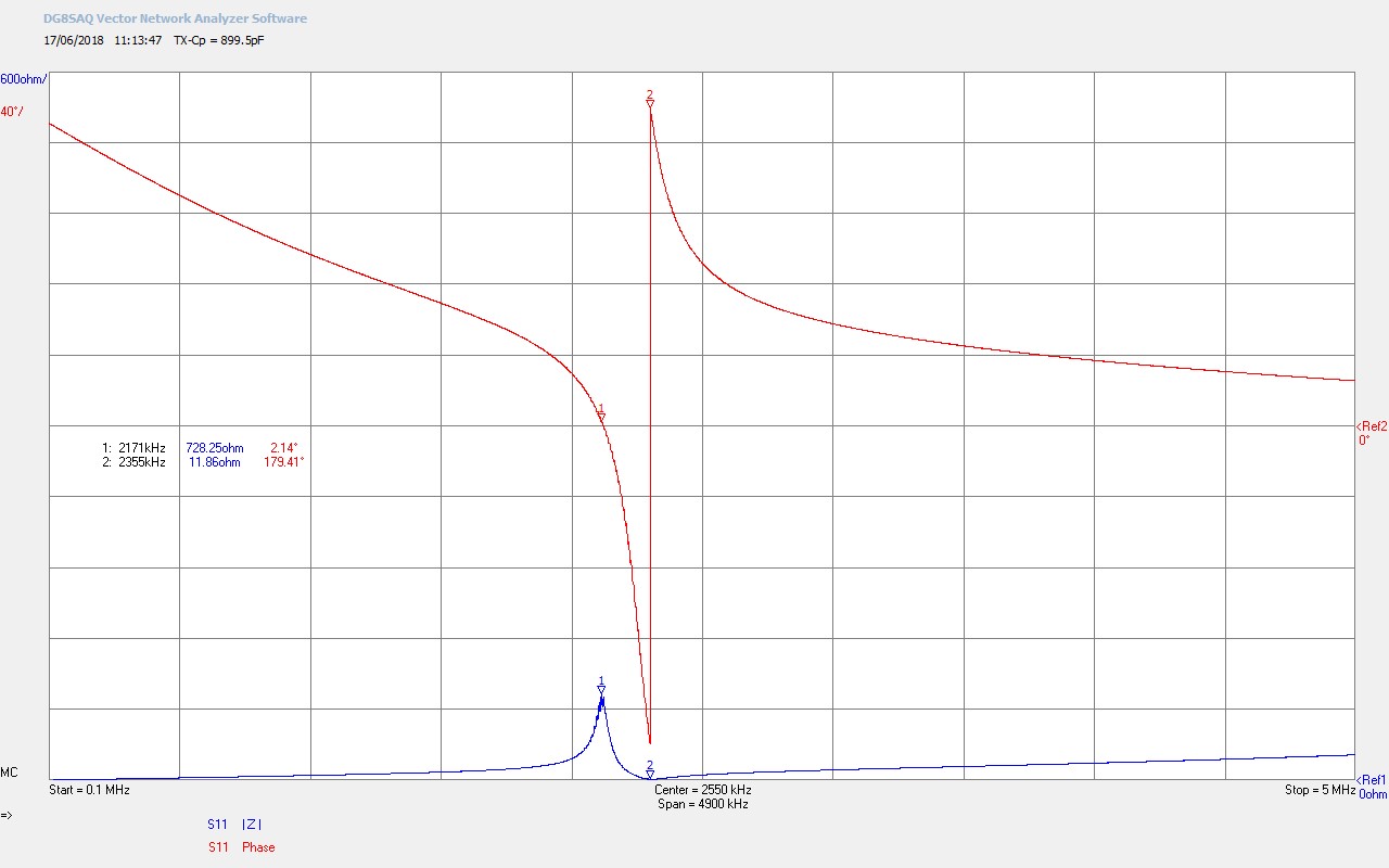
Input impedance Z11, as seen by the generator, of two flat coils bottom-end connected via a single wire cavity in a Tesla Magnifying Transmitter, and tuned to balance the Transverse and Longitudinal modes.
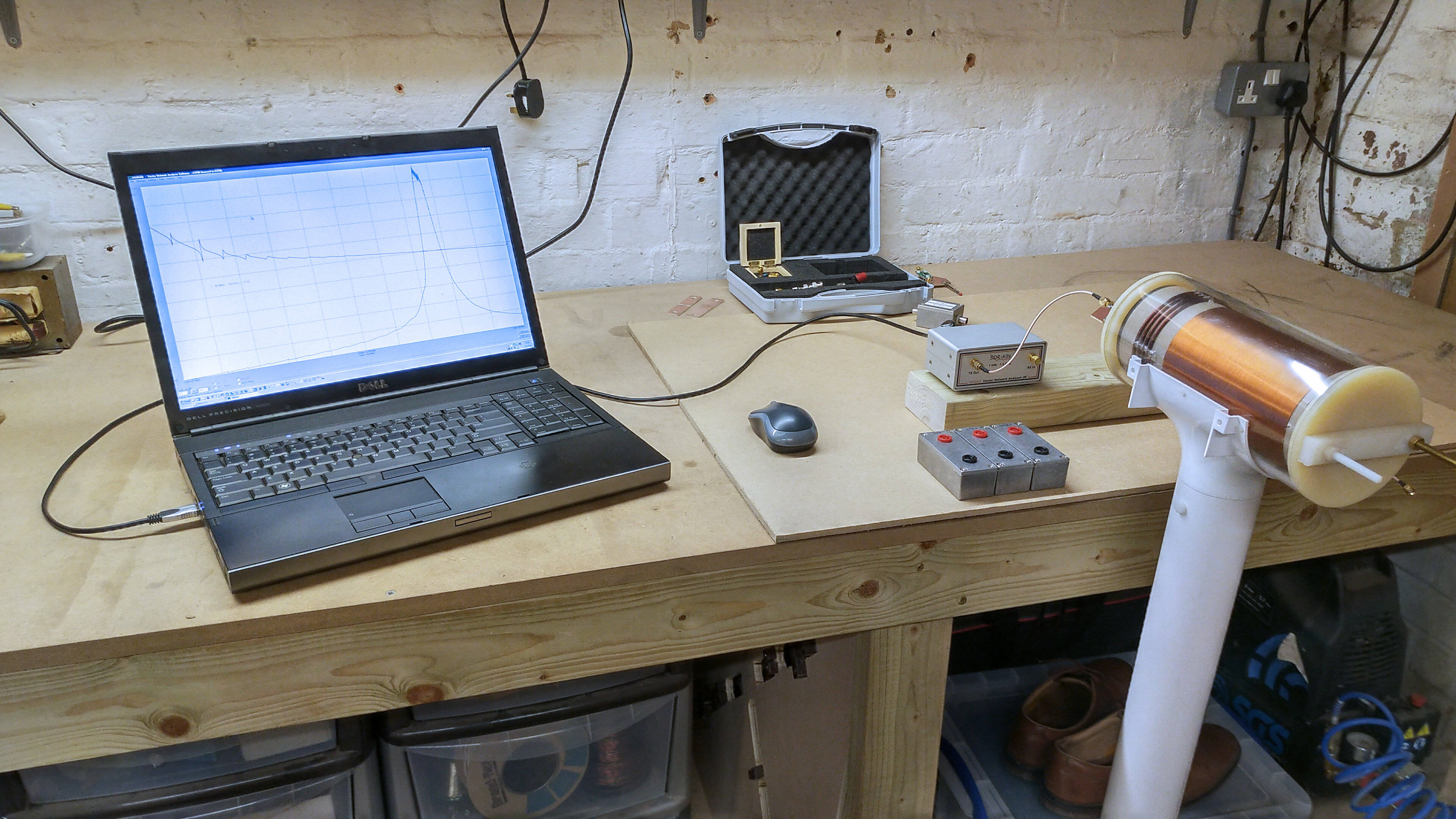
Input impedance frequency measurements of the twin coil experimental apparatus compared on a HP4195A and a SDR-Kits DG8SAQ VNA
Measured upper resonant frequency of oscillation for the single flat coil in Telluric electric power transmission tests.
"Electric power is everywhere present in unlimited quantities ...""Electric power is everywhere present in unlimited quantities and can drive the world's machinery without the need of coal, oil, gas ...""Electric power is everywhere present in unlimited quantities and can drive the world's machinery without the need of coal, oil, gas, or any other of the common fuels."Nikola Tesla c. 1900
In the next sequence of posts the flat coil impedance characteristics are investigated using a range of different measurement methods. Understanding the flat coils impedance charactertistics with frequency is imperative if the coil is to be used optimally, and investigated accurately in experiments regarding the displacement and transference of electric power. Impedance measurements will establish a range of characteristic properties of the flat coil, including:
1. The fundamental resonant frequency of the secondary and the primary, their harmonics, and the effects of close coupling of the two coils.
2. The magnitude and phase of the impedance of the secondary and the primary, and their combination.
3. The effects of electrically loading the secondary and primary.
4. The effects of extending the conductor length of the secondary and primary.
5. Changes in the impedance characteristics when multiple flat coils are joined together.
6. Changes in the impedance characteristics when a flat coil is connected to earth.
7. Suggest bands of frequency that may prove interesting to experiment with the displacement and transference of electric power.
8. Indicate how best to match the flat coil to the required generator for maximum transfer of power.
9. Indicate how best to match the flat coil to the required load or experimental circuit.
The investigation of these characteristics are extensive and will be presented in several parts:
Part 1. Basic resistance and impedance characteristics of a single flat coil where the measurement is either made at dc and single spot frequencies using basic handheld type instruments such as a Digital Multimeter (DMM), LCR meter, and a dip meter.
Part2. Full impedance characteristics (magnitude and phase) with frequency of a single flat coil, measured using a Vector Network Analyser (VNA).
Part3. Full impedance characteristics (magnitude and phase) with frequency of flat coils coupled together in different experimental configurations, and again measured using a VNA.
The specific measurement equipment used in these parts include:
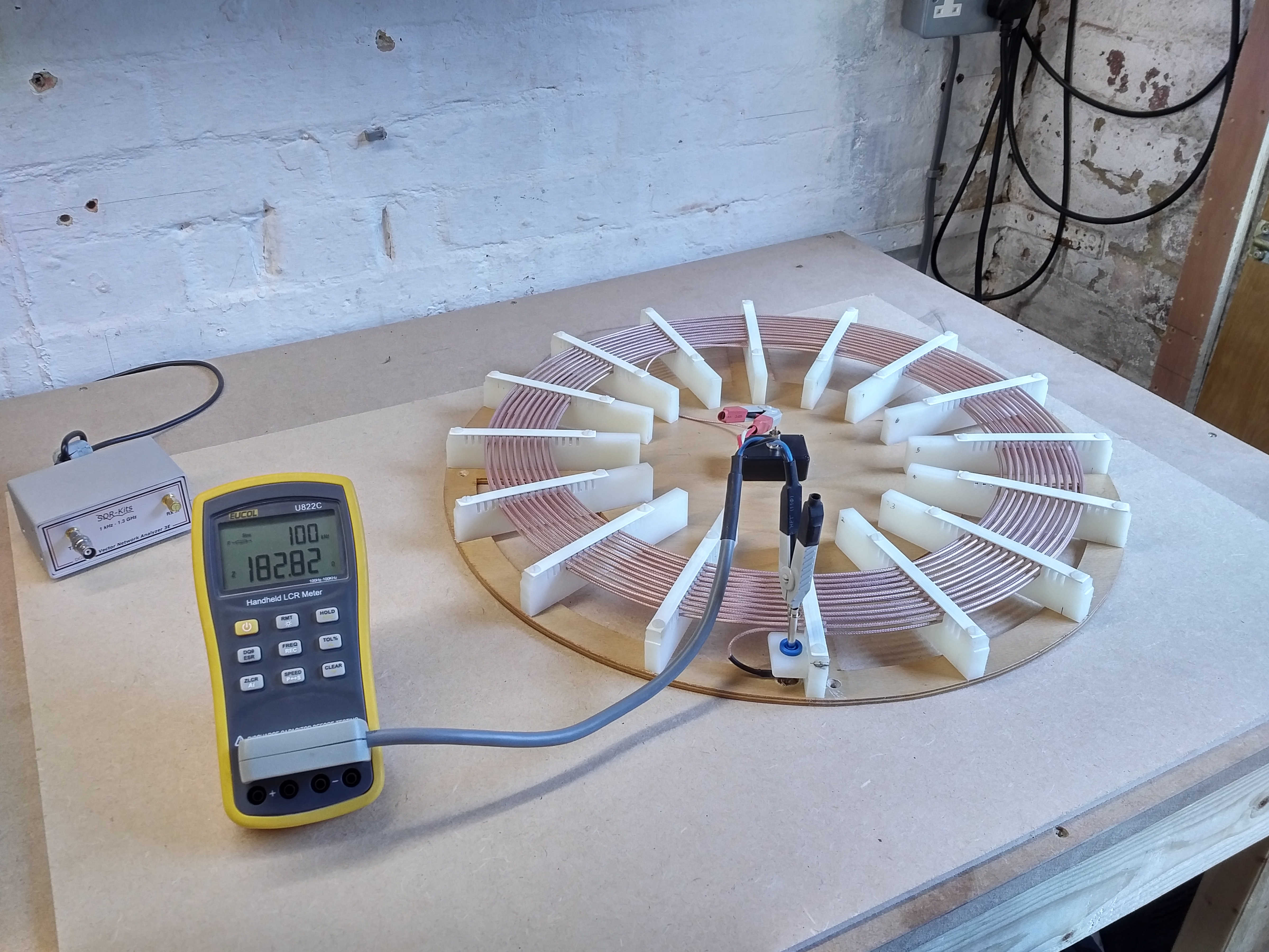
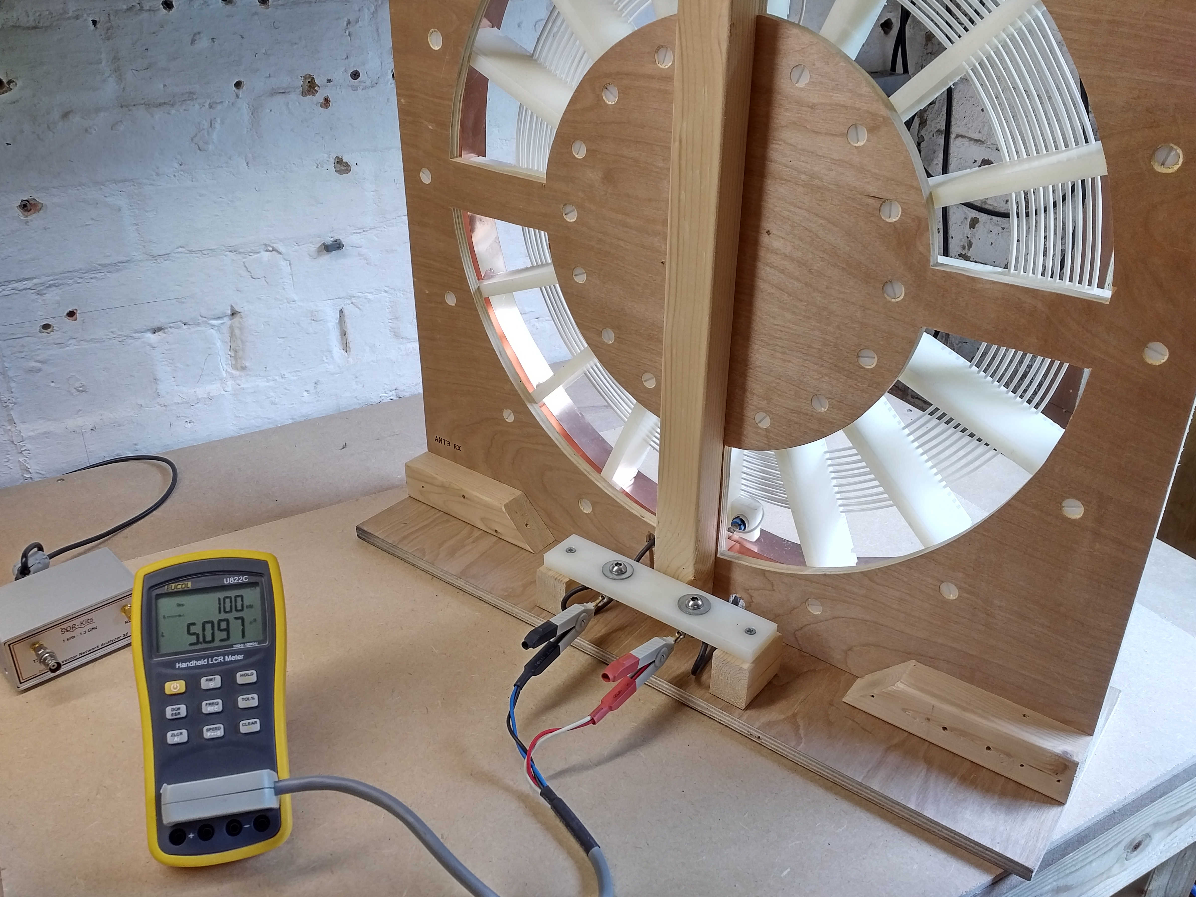
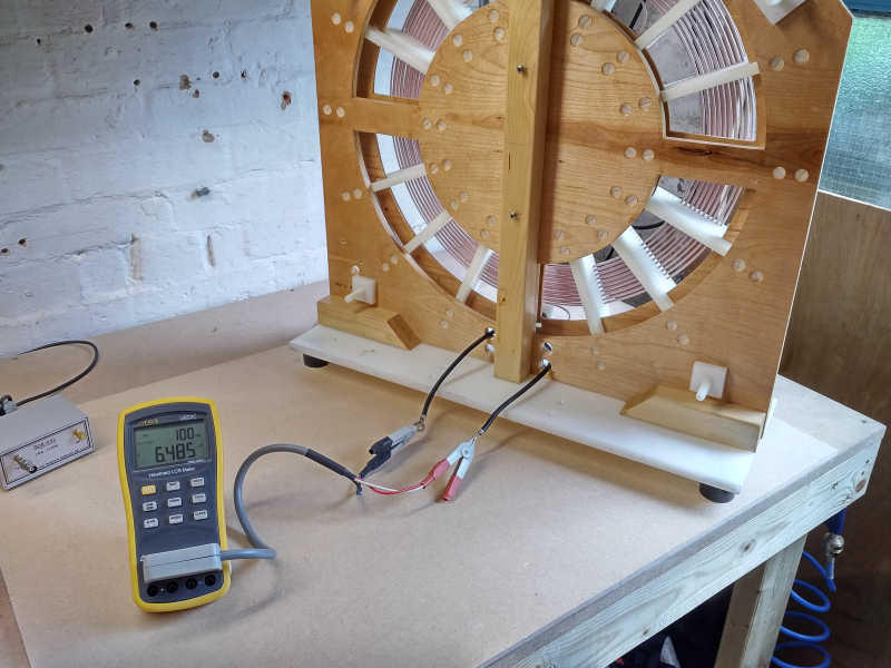
1. Low frequency spot measurements at 100Hz and 100kHz using a Eucol U822C handheld LCR meter (LCR).
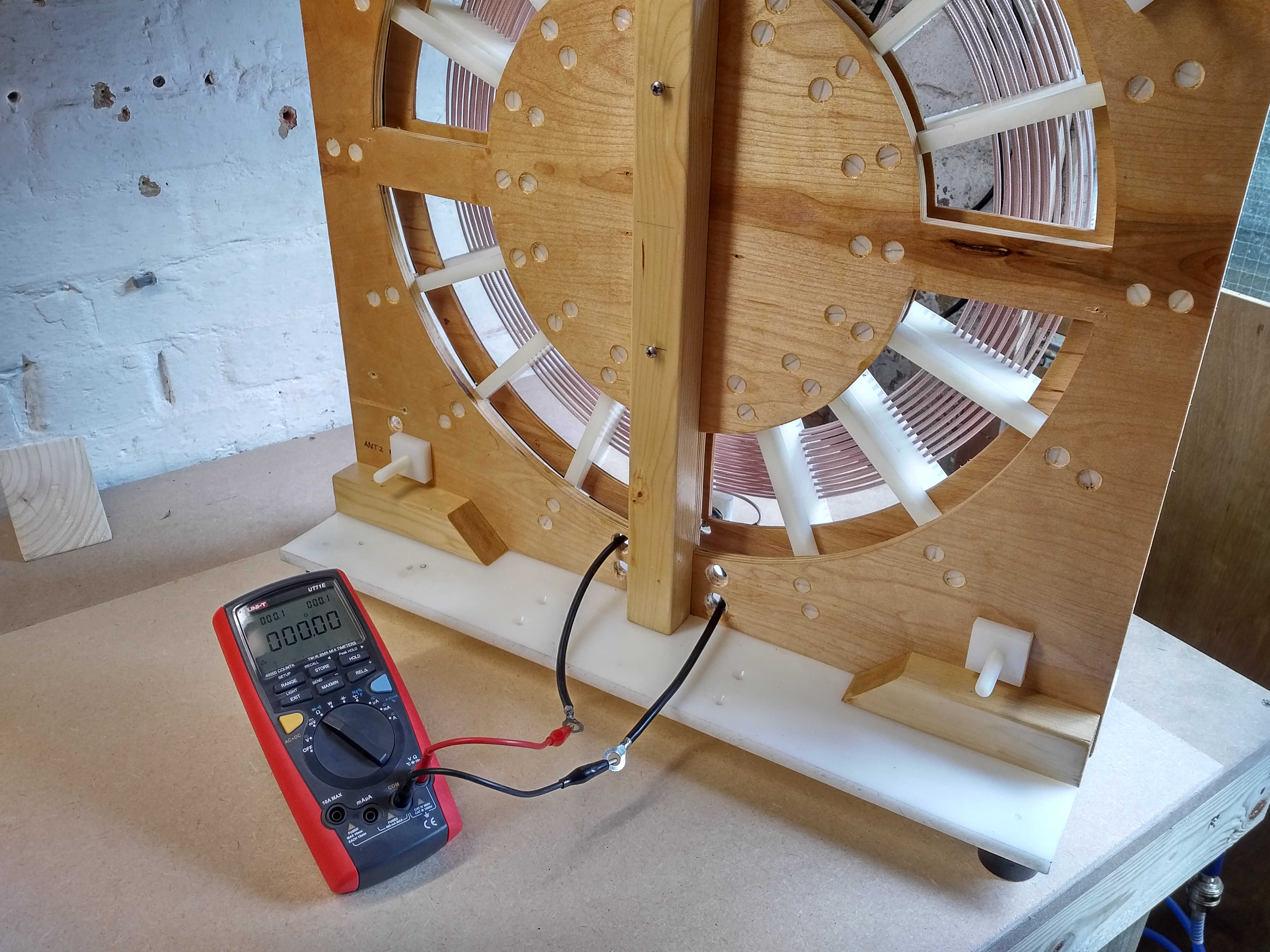
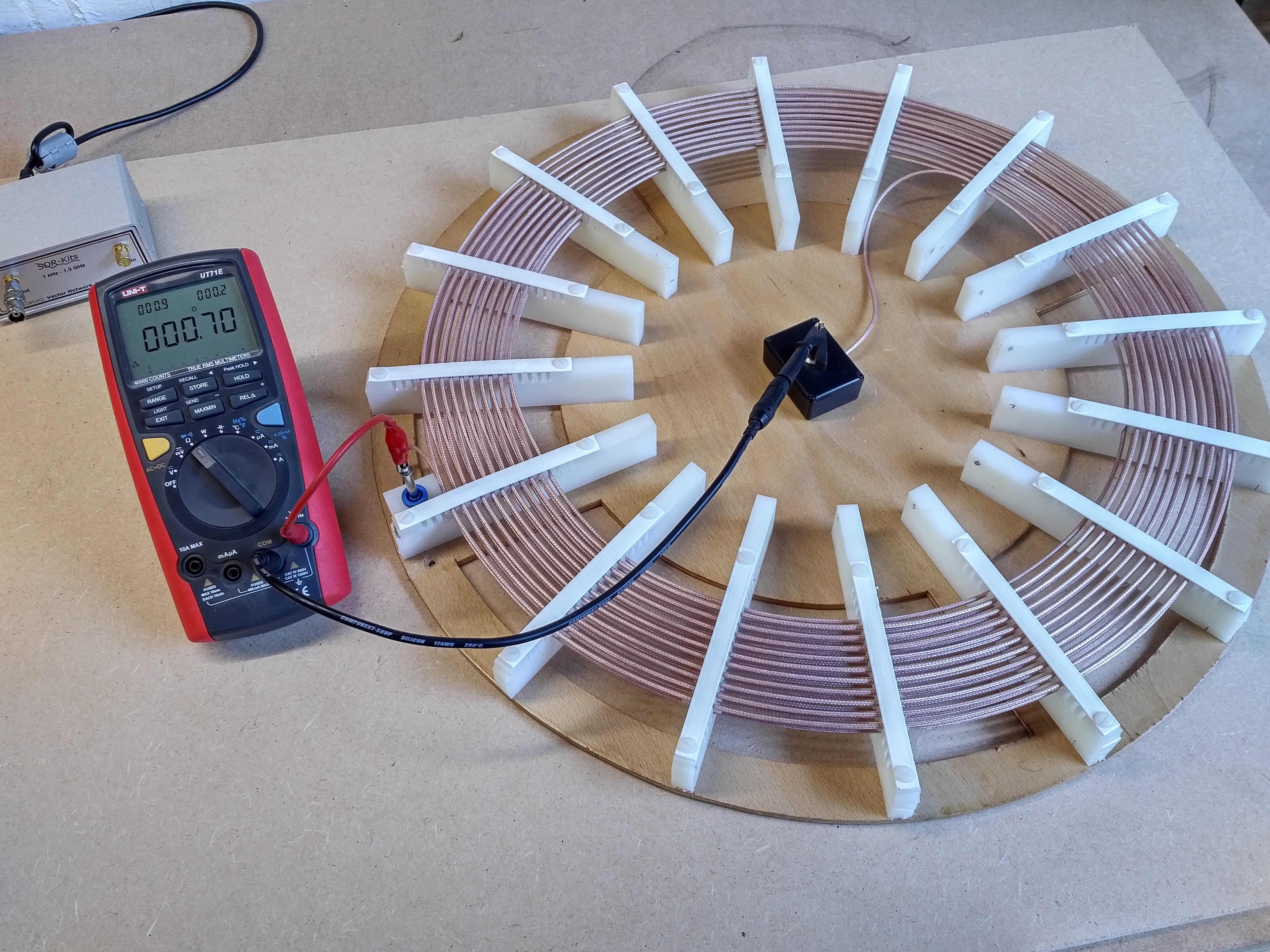
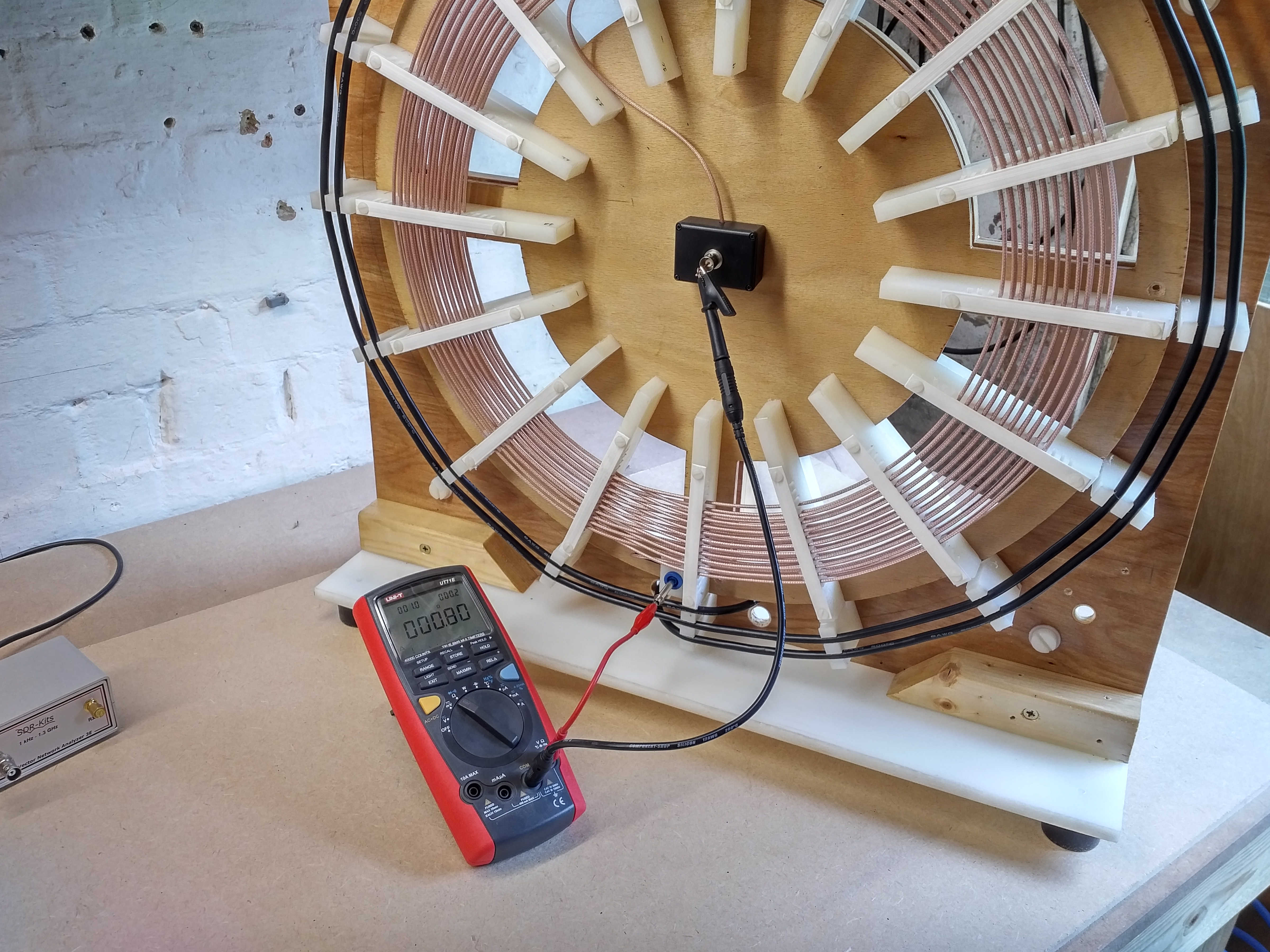
2. DC resistance measurements using a UNI-T UT71E handheld DMM meter (DMM).
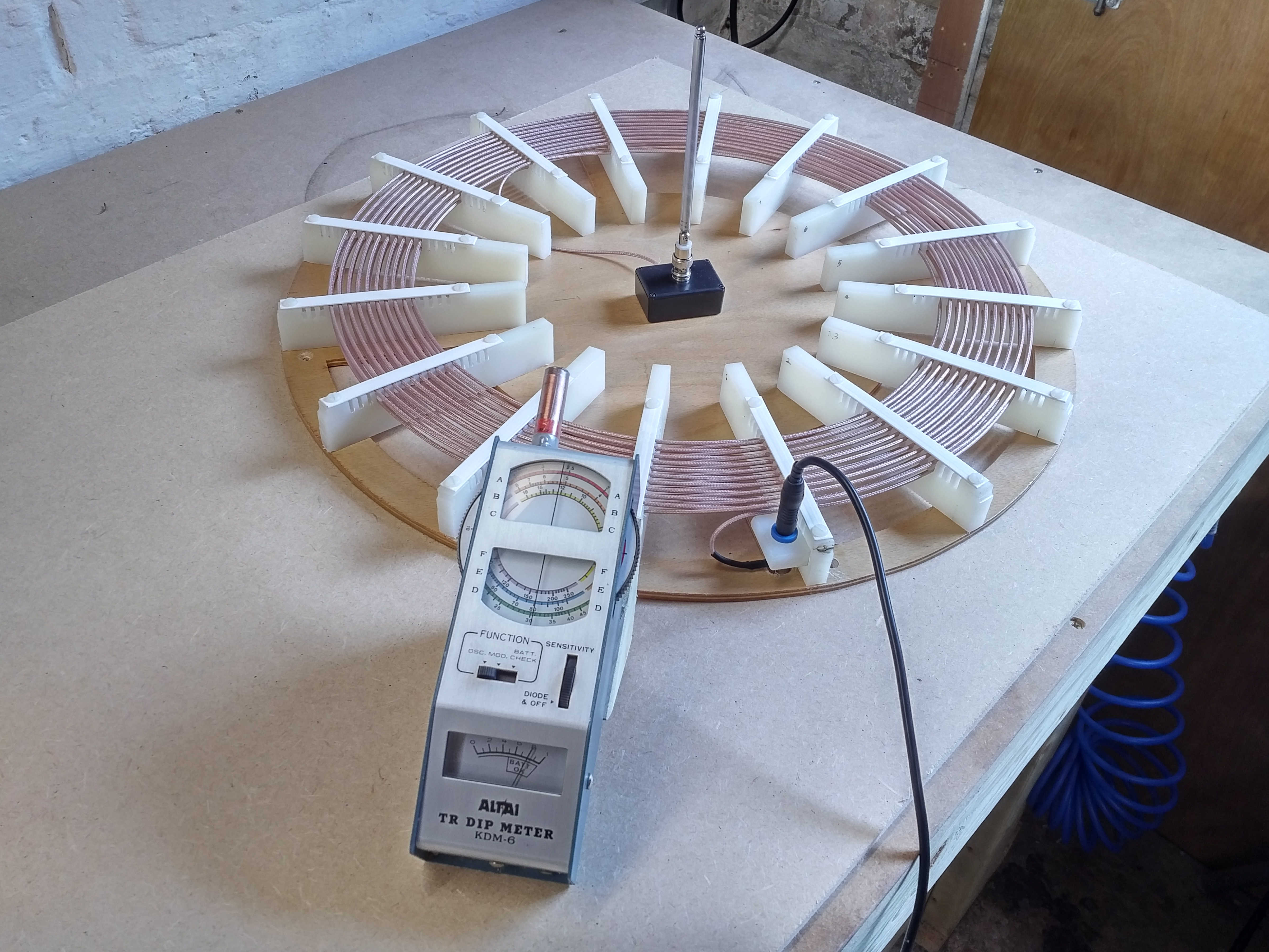
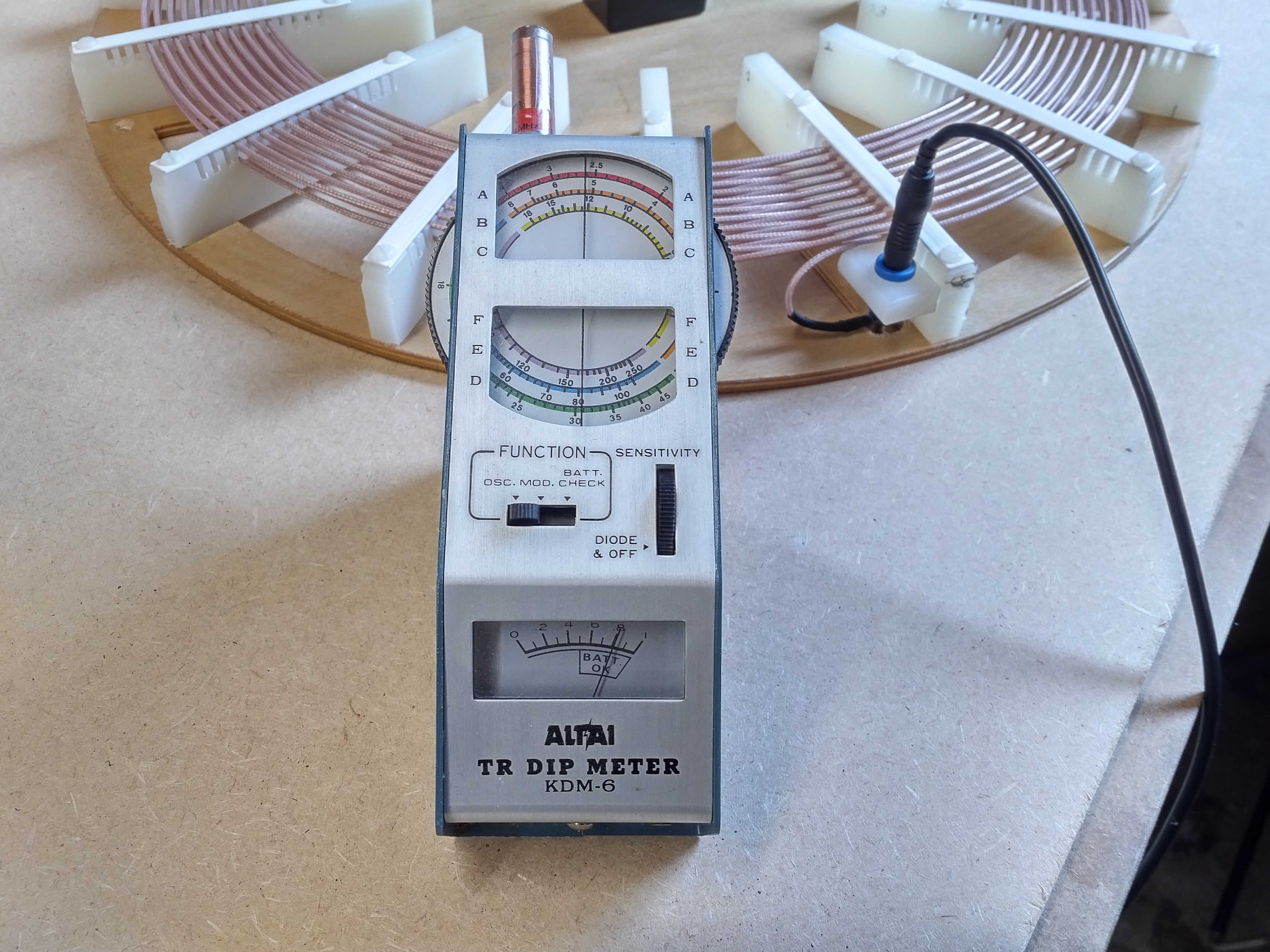
3. Dip meter measurements of the secondary using a Altai TR Dip Meter KDM-6 (DPM)
4. Impedance characteristics using an SDR Kits Vector Network Analyser 3E (VNA-SDR). This VNA has been used for most measurements as it provides data directly connected to a computer, and hence can be more easily displayed and analysed.
5. Impedance frequency scans using a Hewlett Packard 4195A Network Analyser (VNA-HP) mainly to check and confirm the accuracy of the results obtained with the VNA-SDR, and also to use the equivalent circuit function to model actual device circuit equivalent values.
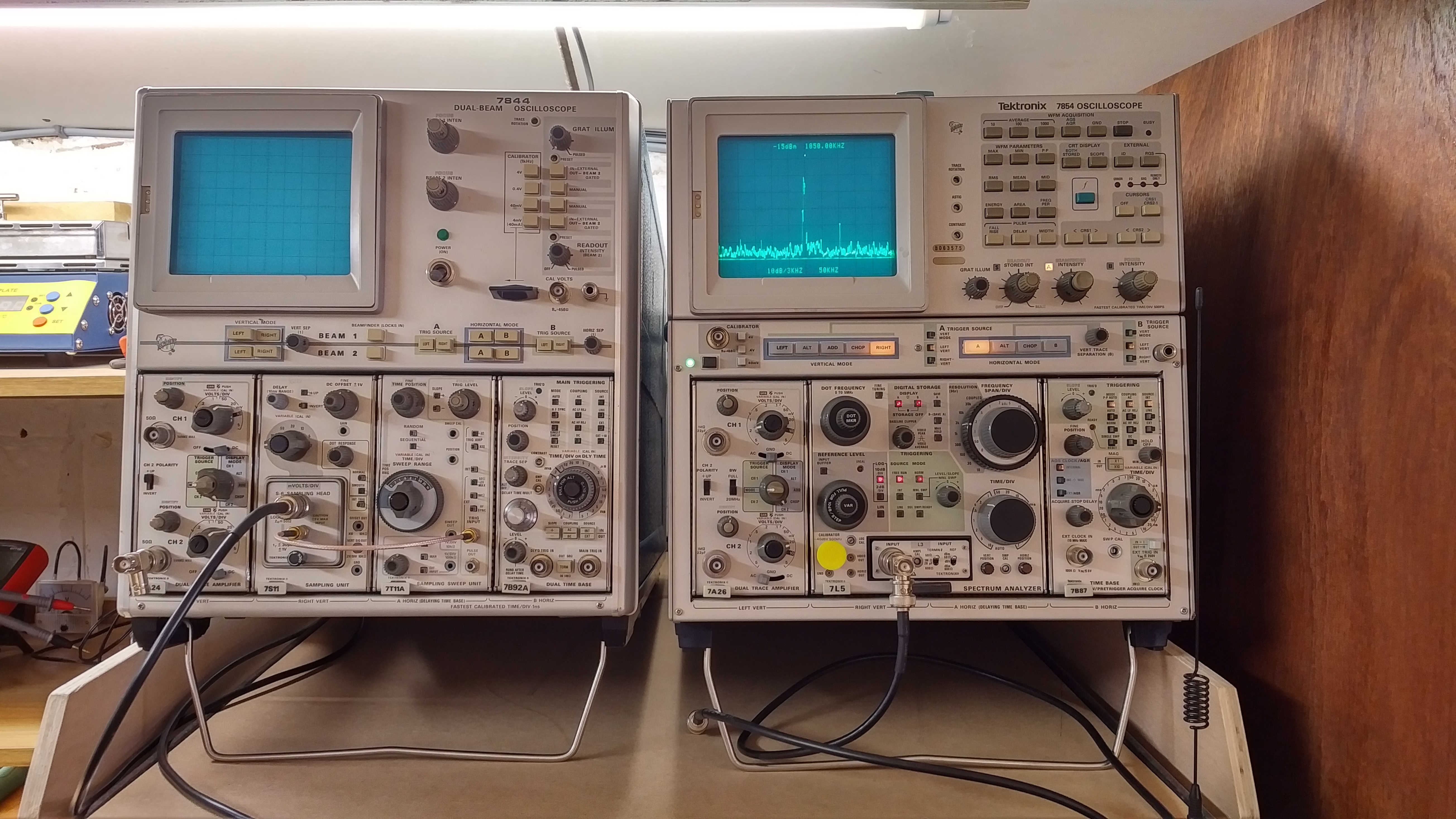
6. Frequency accuracy scans to check the frequencies generated by the DPM, or any other oscillators required, using a Tektronix 7L5 low-frequency spectrum analyser mounted in a Tektronix 7854 mainframe (SPA-TEK).
Each instrument was first calibrated accordingly and tested on a known impedance load or frequency standard in order to confirm accurate measurement. Connection leads were kept short and minimal, and where possible their effects removed by the calibration procedure. At the end of a measurement period the calibration of the instrument was again checked on the same known impedance to confirm stable calibration and measurement.
In this first part the flat coils 3S-1P, and 1S-3P were used. The 3S-1P flat coil has a removable secondary allowing for independent secondary and primary measurements as well as combined, whereas 1S-3P has a fixed secondary and primary.
LCR/DMM Measurements
Figures 1. below show a summary of the measurements made using the LCR and DMM, and the full data is summarised further below.
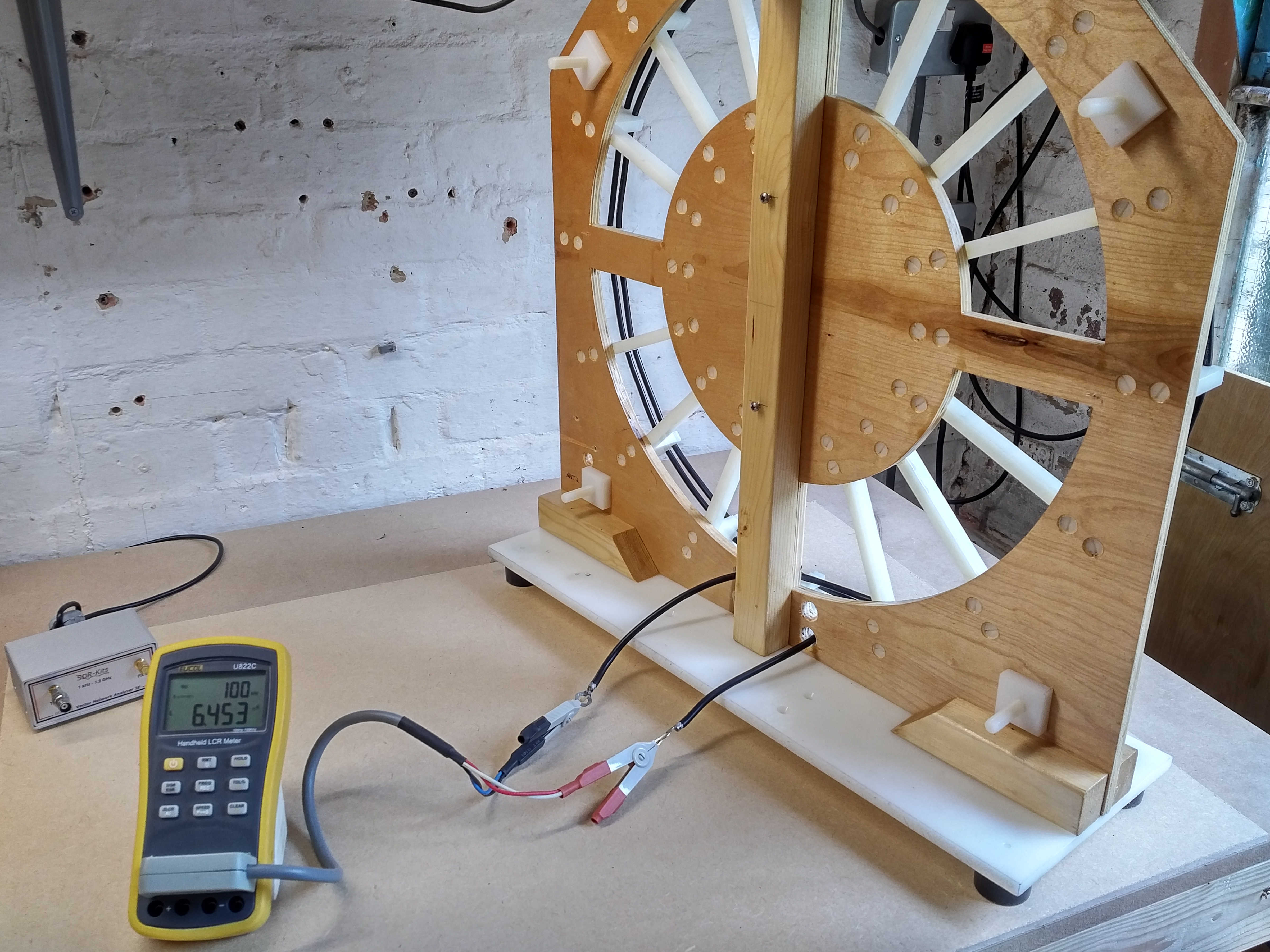
Fig. 1.1. 1P primary inductance 6.453µH @100kc/s.
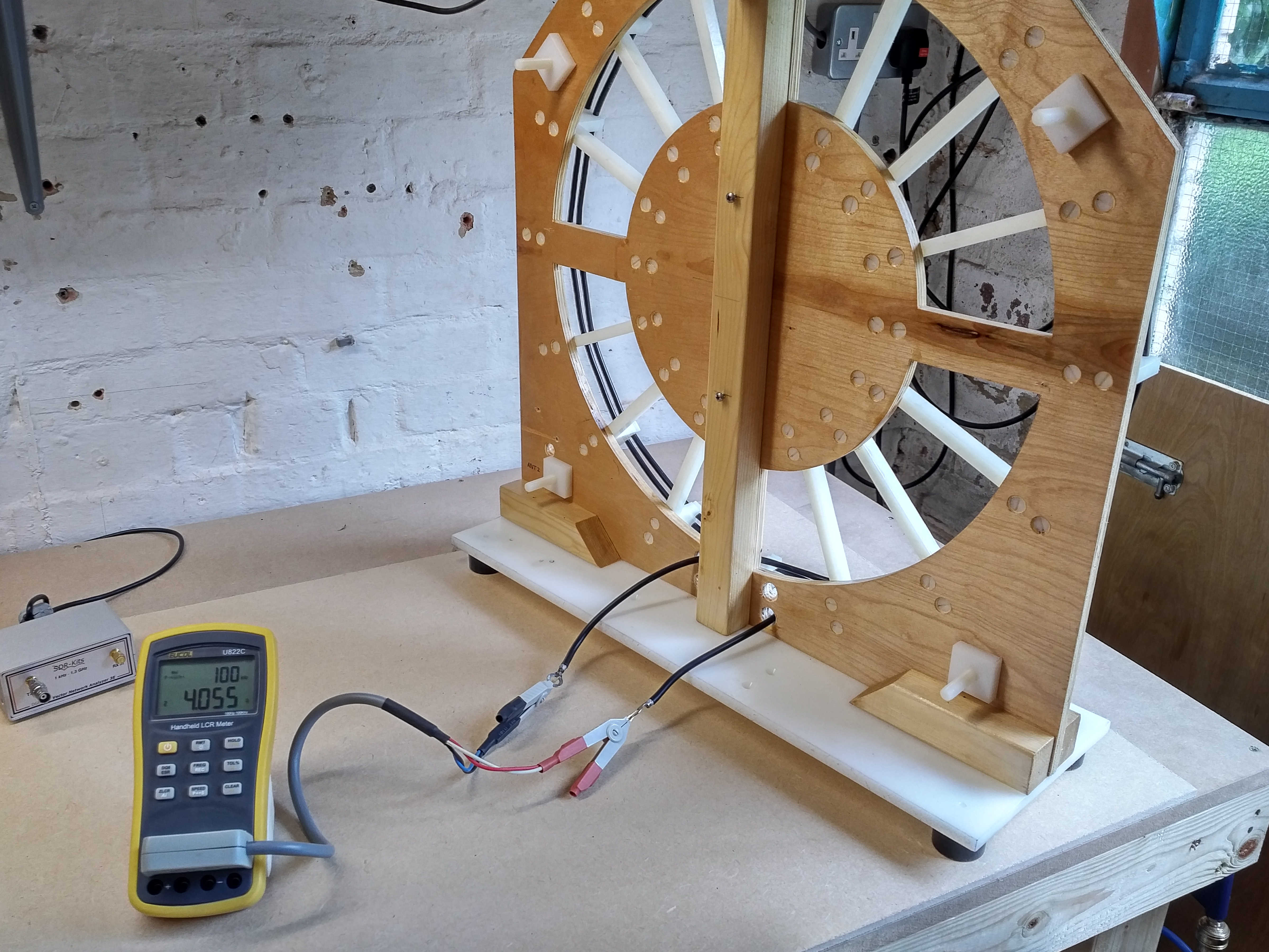
Fig. 1.2. 1P primary impedance 4.055Ω @100kc/s.
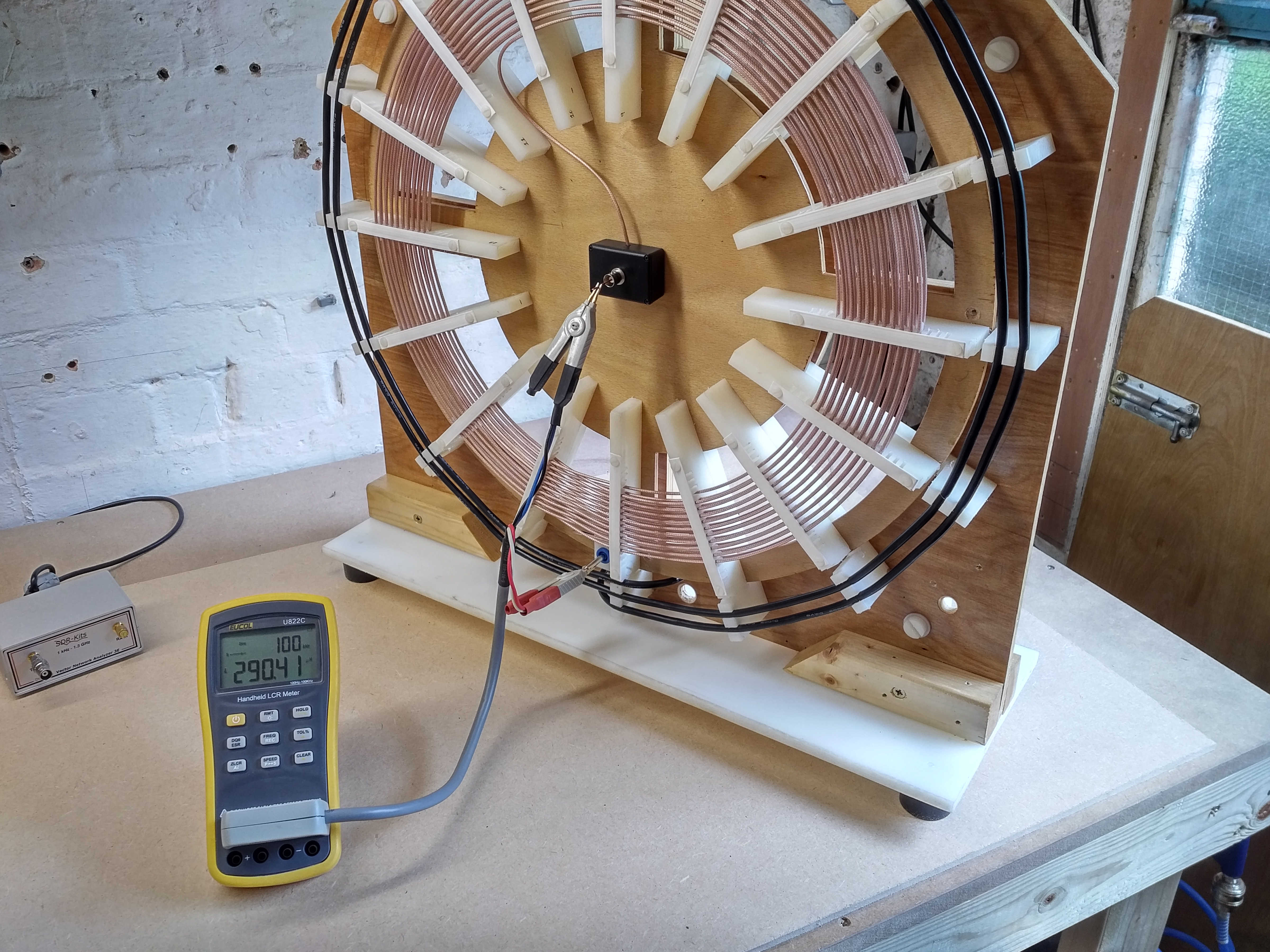
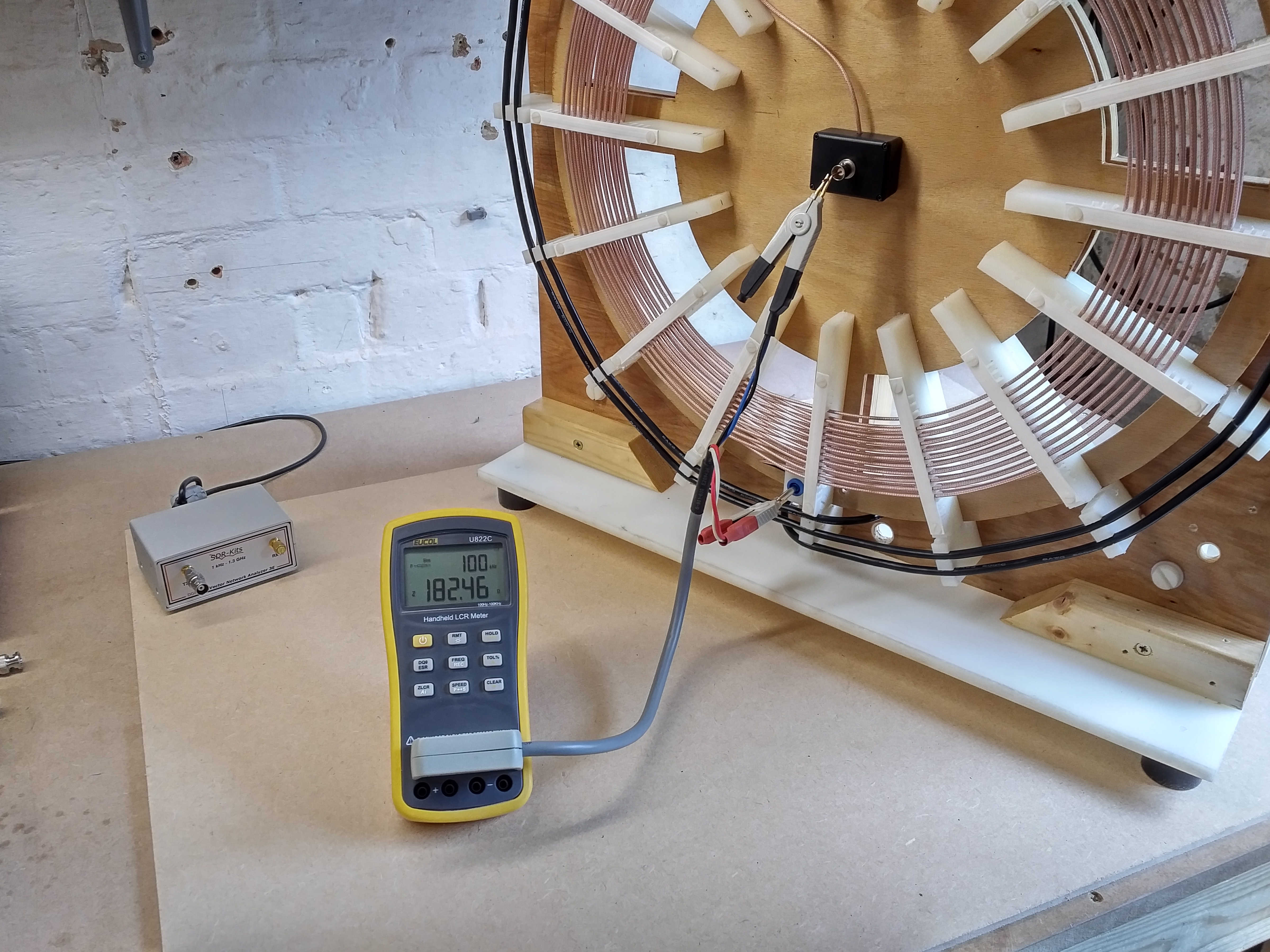
Fig. 1.3. 3S-1P primary inductance has increased slightly with addition of 3S secondary to 6.485µH @100kc/s.
Summary of the LCR/DMM results and conclusions so far:
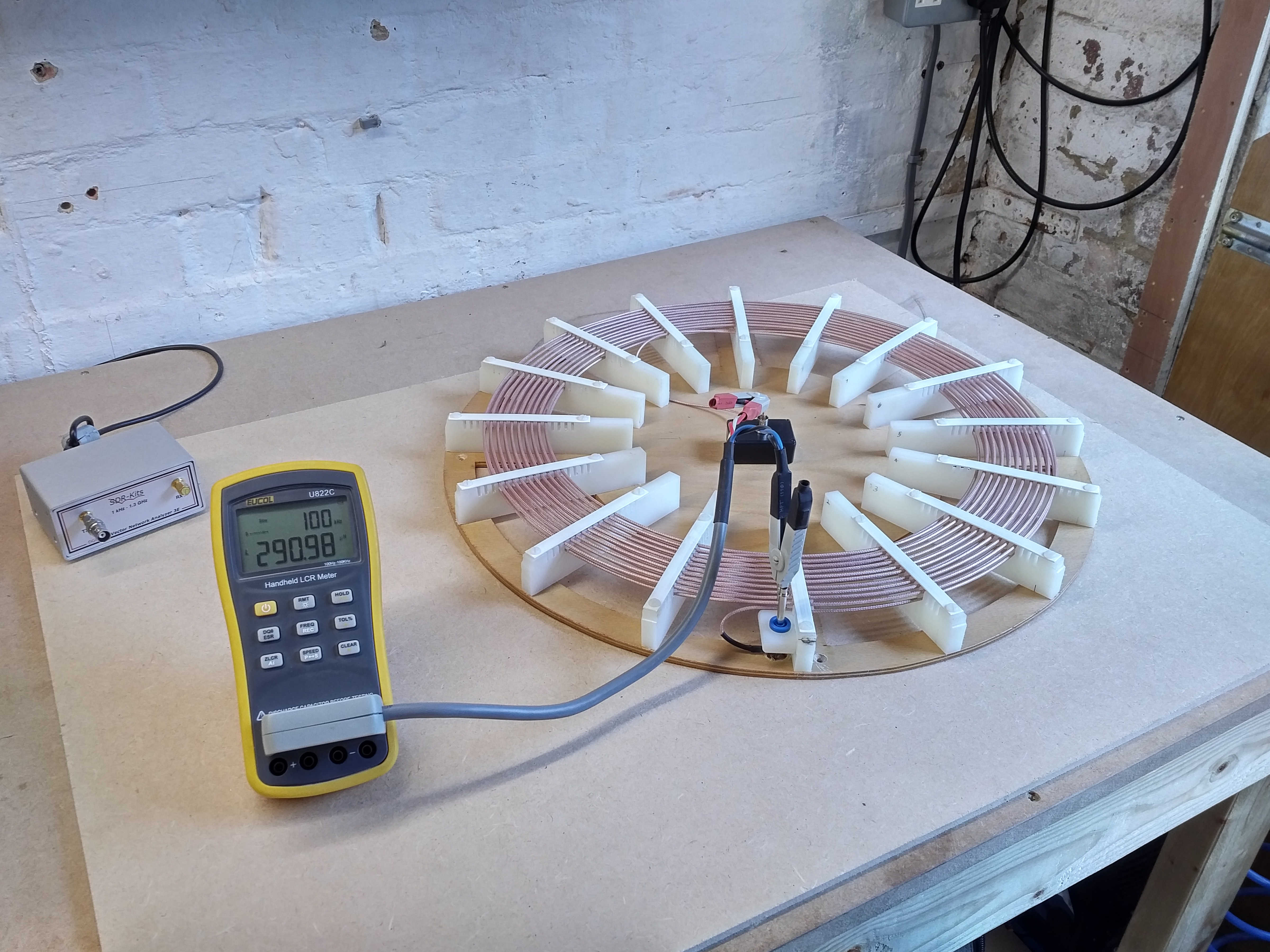
1. The secondary inductance indicated from the flat spiral coil calculator in Part 1 of the design was (2 x 71.419µH for an upper and lower coil) = 142.84µH. From the basic spot measurements we find that the actual inductance of the secondary is almost double for both types of coils 1S (298.36µH) and 3S (290.98µH). The coil calculator assumes a solid conductor, and is also not designed to account for the specialised inter-leaving that has been used to construct the upper and lower turns of the secondary. It is also unclear what model the calculator is using to calculate inductance for the spiral conductor. It is concluded that the flat spiral coil calculator is useful for the mechanical design of the secondary but not in predicting the inductance of the coil for an inter-leaved secondary in this case.
2. The primary inductance indicated from the flat spiral coil calculator in Part 3 of the design was 4.811µH. From the basic spot measurements we find that the actual inductance of the 3P primary (copper strip) is closer to that predicted at 5.097µH (+5.9% error) showing that the coil calculator can more accurately calculate the inductance in a simple case of a small number of turns with a solid conductor. In the case of 1P primary (silicone coated micro-stranded cable) again the conditions are more difficult and the inductance increases away from that expected from the design, measuring 6.453µH (+34.1%). It is concluded that the flat spiral coil calculator is useful for the mechanical design of the secondary but not in predicting the inductance of the coil for complex cable materials and geometry.
3. The slight decrease in inductance and impedance of the 3S secondary when added to the 1P primary to make the 3S-1P flat coil indicates a loose coupling between the two coils of < 0.25, which is best suited to establishing a resonant cavity in the secondary, and hence to experiments in to the displacement and transference of electric power.
4. The impedance and resistance of the primary in both cases 1P and 3P is low, and hence suitable for the generator to pass large oscillating and transient currents which will be needed to drive the flat coil in the intended experiments.
5. The magnitudes of inductance, impedance, and resistance of the secondary and primary appear to be generally in the correct region for the intended experiments. A clearer view of the frequency characteristics and impedance matching requirements will be established in part 2.
DPM Measurements
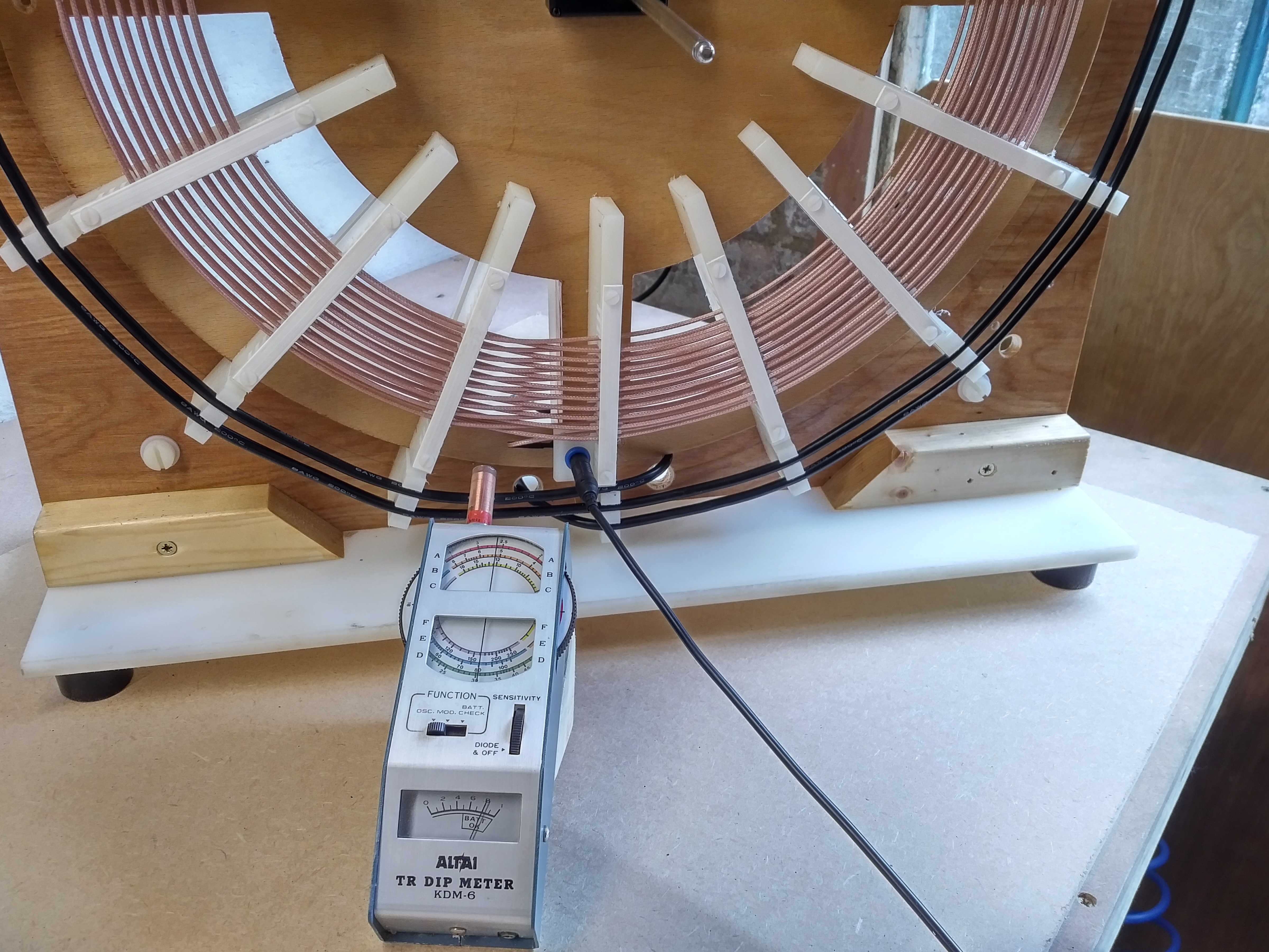
For dip meter measurements a 180cm lead was added to the outer or bottom-end coil terminal in order to lower the impedance sufficiently for λ/4 measurements. As the dial of the dip-meter is not a very accurate scale the oscillator setting was checked for frequency using the Tektronix 7L5 spectrum analyser with a small pick-up antenna.
For 3S-1P results a short telescopic aerial fully retracted 15cm long was added to the central coil terminal, which is to allow for fine wire length tuning during telluric reception experiments.
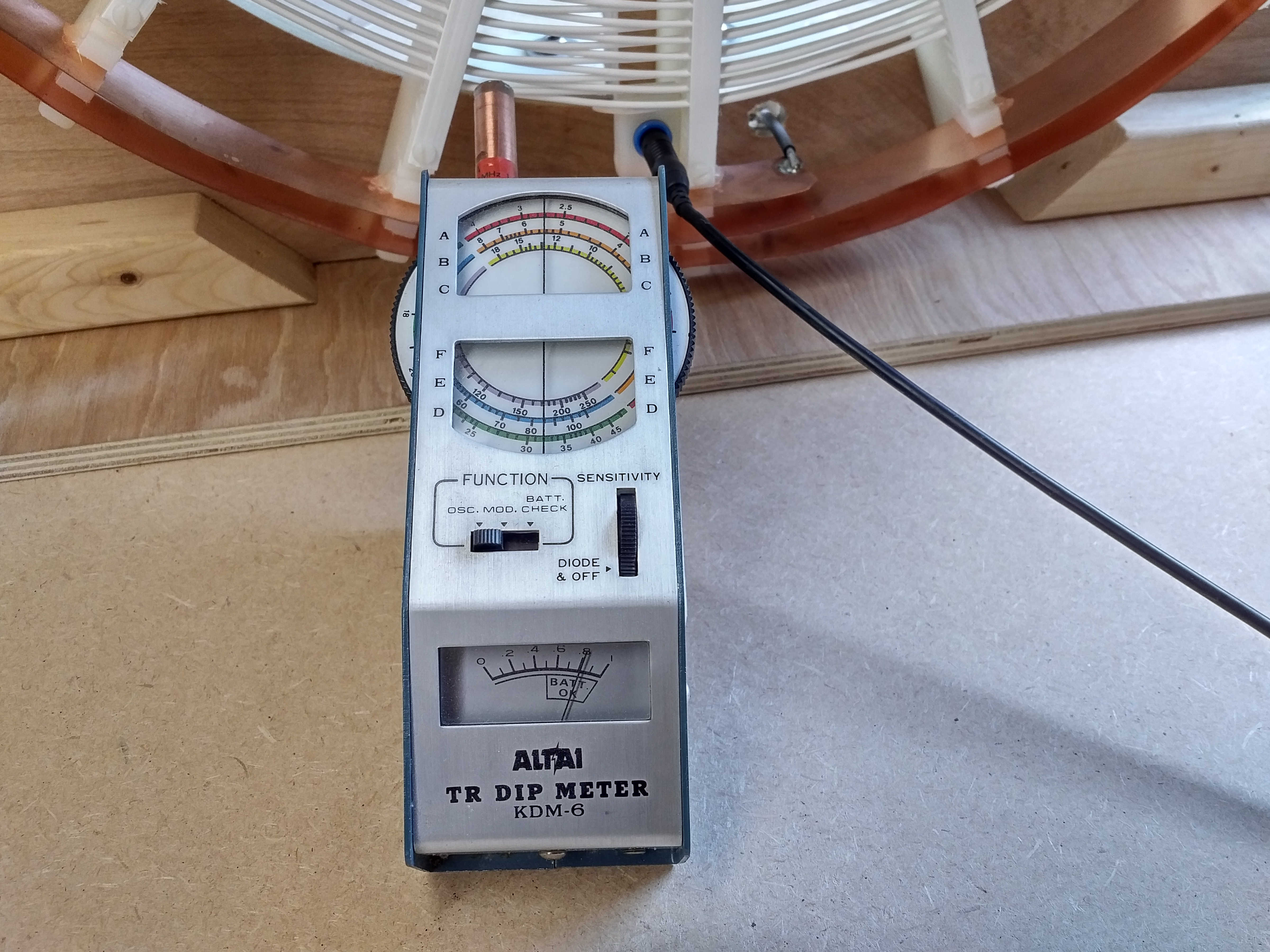
For 1S-3P results a ceramic bulb holder and a neon bulb was added to the central coil terminal, which will be used in experiments in the displacement and transference of electric power.
Figures 2. below show a summary of the measurements made using the DPM, and the full data is summarised further below.
Fig. 2.1. 3S secondary fundamental resonant frequency measured with a dip meter (DPM), 2625kc/s on scale A (red).
Fig. 2.2. 3S secondary fundamental resonant frequency 2625kc/s.
Fig. 2.3. 3S-1P secondary fundamental resonant frequency has reduced slightly when the primary is added, 2605kc/s.
Fig. 2.4. 1S-3P secondary fundamental resonant frequency 2730kc/s.
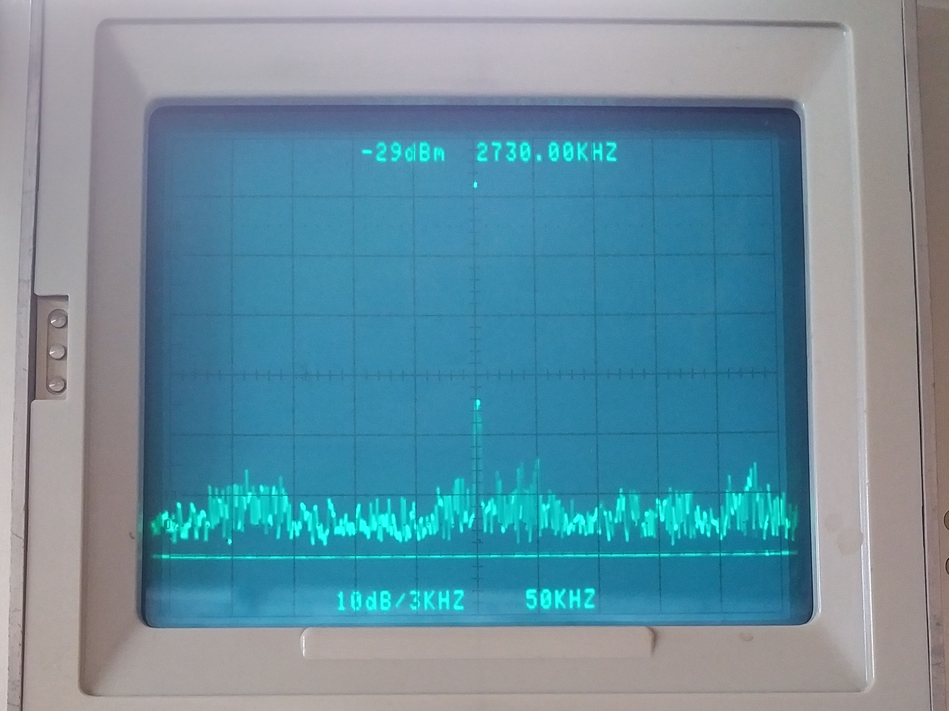
Fig. 2.5. Checking the DPM oscillator output using a Tektronix 7L5 spectrum analyser and small pick-up antenna. The DPM oscillator is set to the 1S-3P measurement in the previous fig. 2730kc/s.
DPM Measurements for 3S-1P Secondary
With the secondary 3S removed:
Frequency of dip meter maximum: 2625kc/s
With the secondary 3S added:
Frequency of dip meter maximum: 2605kc/s
DPM Measurements for 3S-1P Secondary
Frequency of dip meter maximum: 2730kc/s
Summary of the DPM results and conclusions so far:
1. The frequency at which a 180° phase change due to the λ/4 wire length was designed at 2400kc/s in part 1 of the design. In the dip-meter measurement the coil is very loosely coupled to the meter, and so the secondary is very lightly loaded where the point of maximum impedance of the parallel resonant circuit will occur very close to the 180° phase change. The results of 2625kc/s for 3S and 2730kc/s for 1S are higher than expected from the simple calculation from wire length in part 1 of the design, but may also indicate other influences on the fundamental resonant frequency such as the inter-winding capacitive network of the coil.
2. The effect of the 3S added to 1P to form the 3S-1P flat coil shows a slight loading from the primary on the secondary and hence reducing the resonant frequency from 2625kc/s to 2605kc/s. This is again indicative of a loosely coupled coil suitable for the intended experiments.
3. It was not possible to identify any harmonic resonant frequencies above the fundamental using the DPM. It is most likely that the harmonics are much smaller in amplitude than the fundamental, and that the method of tuning the DPM is not sufficiently sensitive to detect and indicate the very small harmonic changes.
4. The basic frequency points derived from the DPM are generally in the correct region for the intended experiments. A much clearer view of the frequency characteristics will be established in part 2.
Click here to continue to the flat coil frequency measurements part 2.
1. A & P Electronic Media, AMInnovations by Adrian Marsh, 2019, EMediaPress
2. Dollard, E. and Energetic Forum Members, Energetic Forum, 2008 onwards.
In this second part full input, small signal, impedance characteristics Z11 (magnitude and phase) with frequency of a single flat coil are measured using a Vector Nework Analyser (VNA). The SDR-Kits Vector Network Analyser 3E (VNA-SDR) is predominantly used as it provides data directly connected to a computer. Some measurements have also been cross-measured and checked using a Hewlett Packard 4195A Network Analyser (VNA-HP), and particularly when an equivalent circuit function is required to model actual device circuit equivalent values.
The measurements reported in this second part are for Z11, the effective input impedance that the generator will see when connected to the input of the flat coil, and subsequently in part 3 connected with a range of loads and other flat coils. Impedance measurements for Z21 the transmission impedance between the input of the primary and the output of the secondary will be reported in future parts.
For network analyser impedance-frequency measurements an adjustable capacitance box was connected across the primary coil at the correct termination point to match the equal weights of copper for the secondary and primary. The unconnected load capacitance of the box when set to 0pF is 30.5pF. The VNA being used was calibrated to the end of the coaxial cable to be connected to the capacitance box and then tested with a 50Ω termination for accuracy over the frequency range. This calibration was then re-checked at the end of the measurement cycle to confirm stable calibration throughout the measurement period.
A wider band frequency scan 0.1MHz – 20MHz was used initially in order to identify the fundamental resonance frequency, any low-order harmonics, and any other impedance features of interest. Subsequently the frequency scan band was reduced to (0.1MHz – 5MHz) to allow for greater detail in the results.
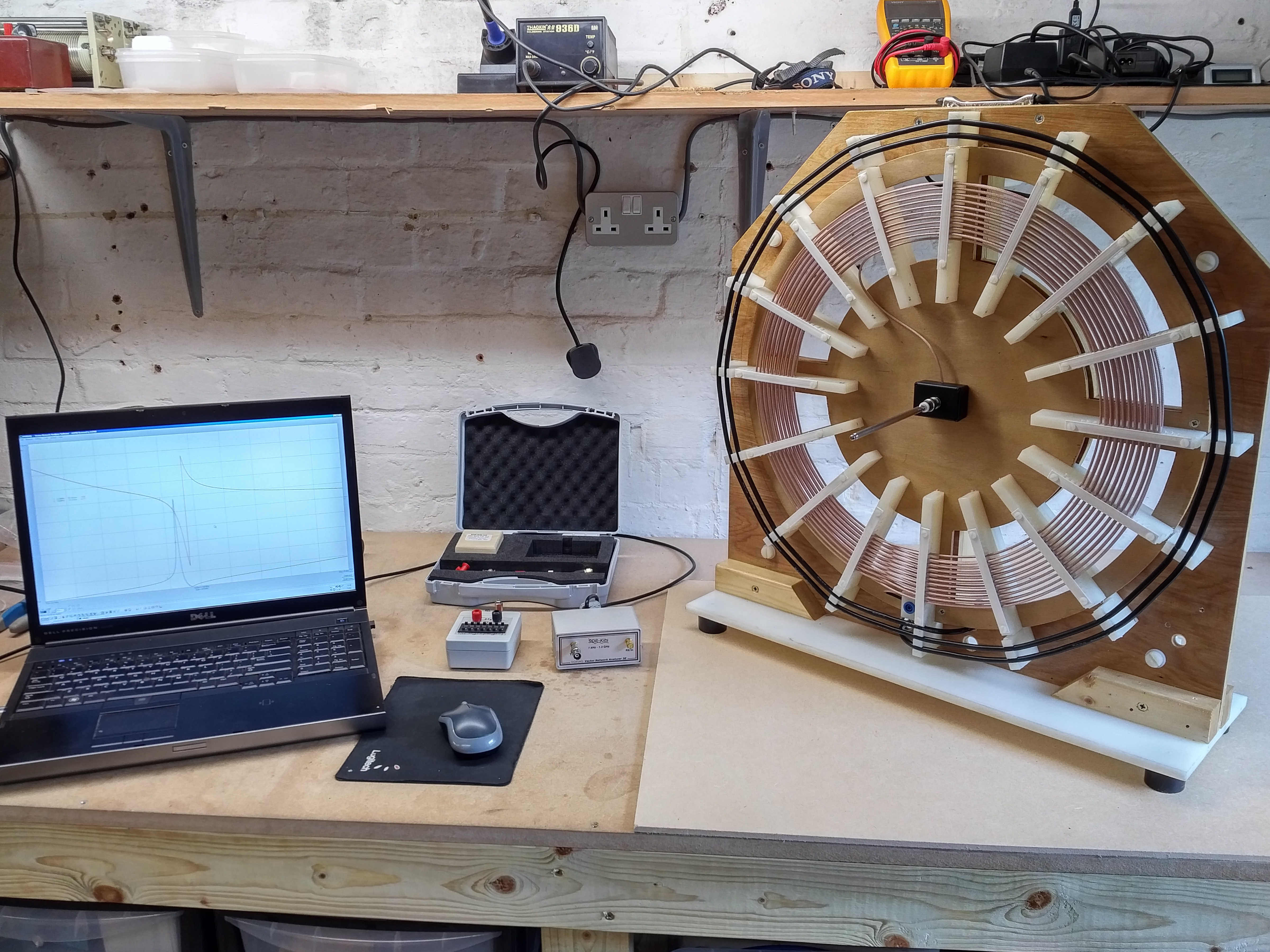
Figures 1. show the measurement arrangement.
Fig. 1.1. Measurement setup for VNA-SDR measurements on flat coil 3S-1P.
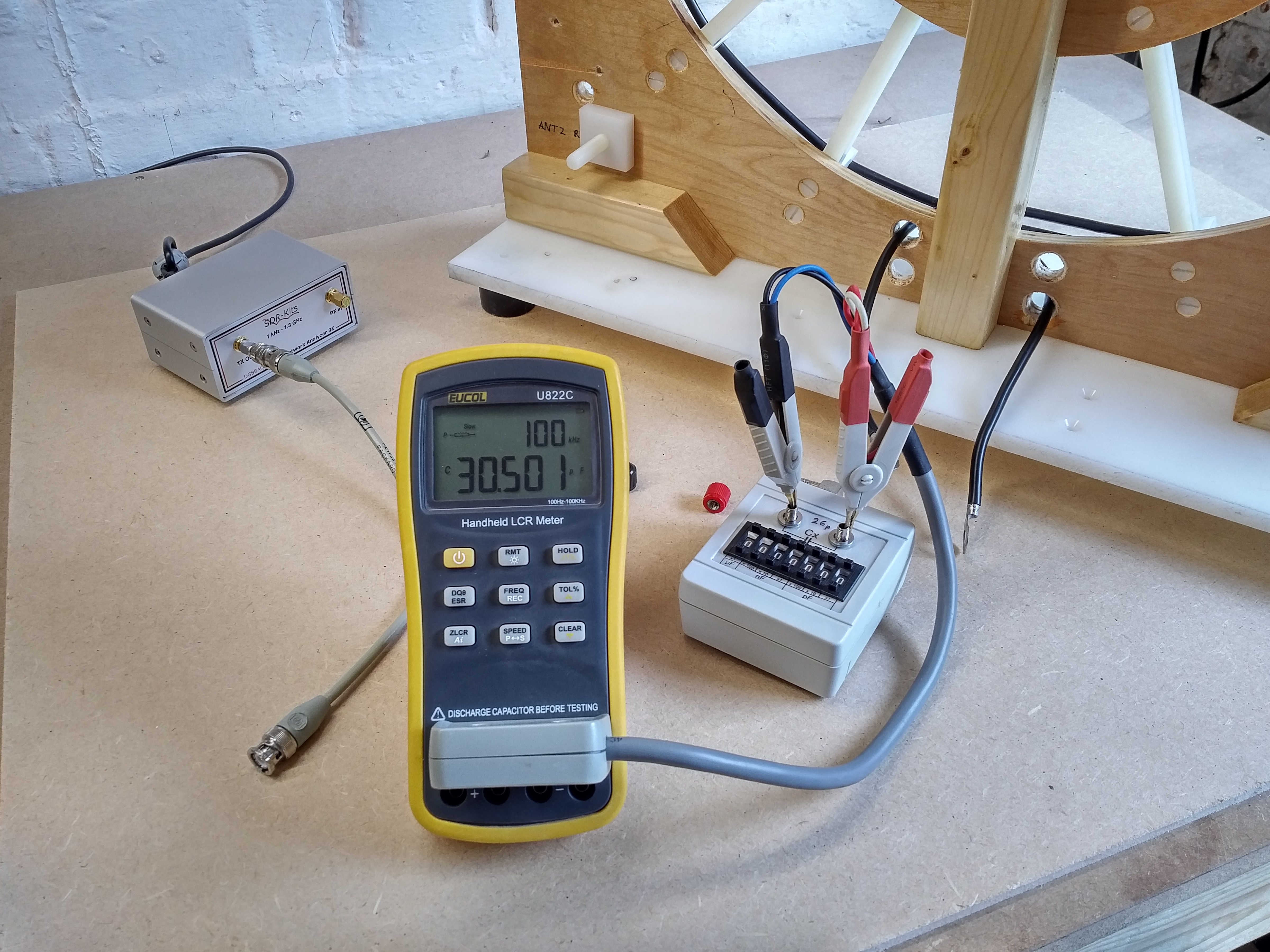
Fig. 1.2. Measuring the parasitic loading capacitance of the capacitance box when set to 0pF, and to be used for flat coil tuning in the VNA impedance measaurements, 30.5pF @100kc/s
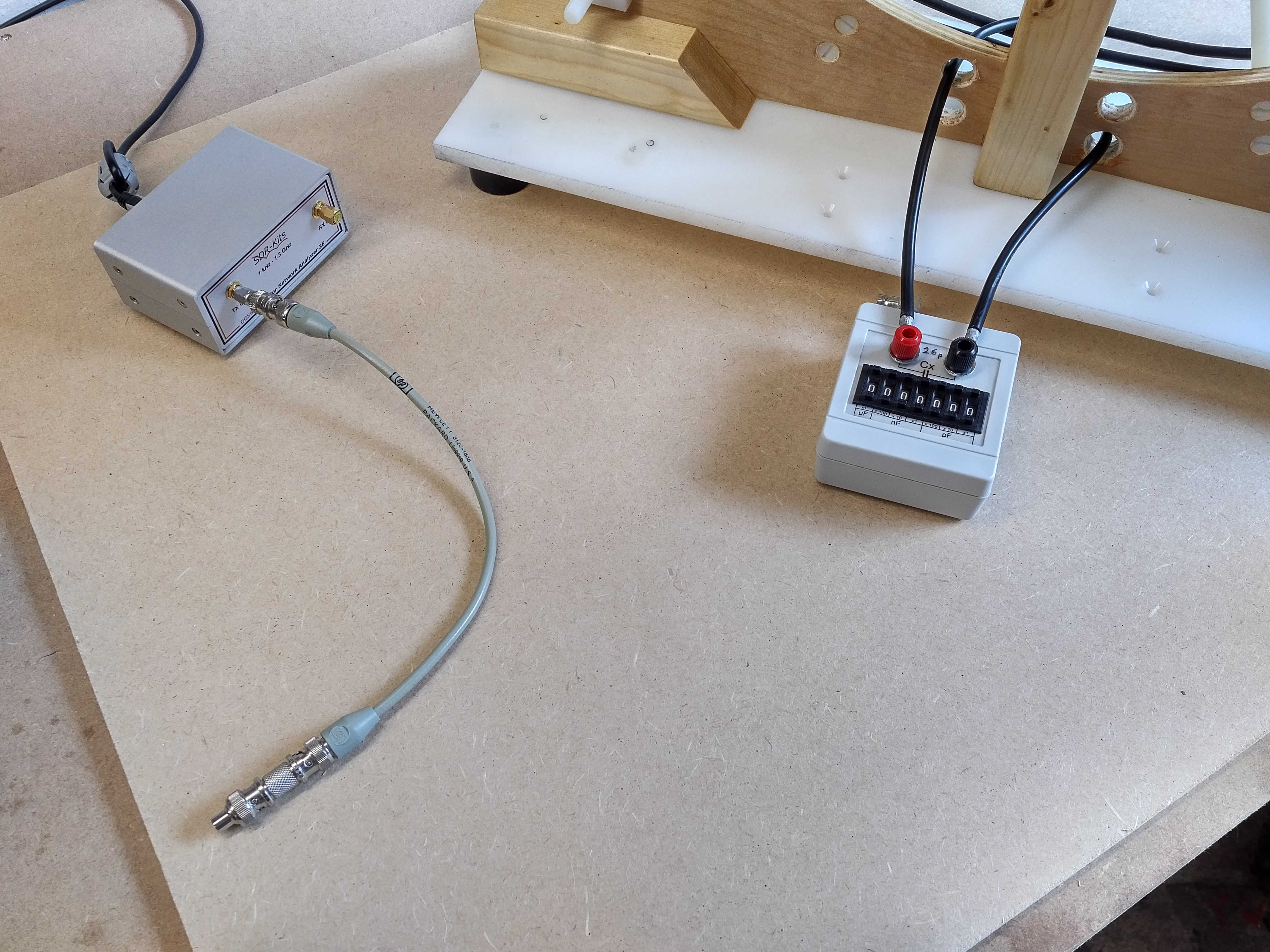
Fig. 1.3. Calibrating the VNA to the end of the connection wire to be connected to the output of the capacitance box.
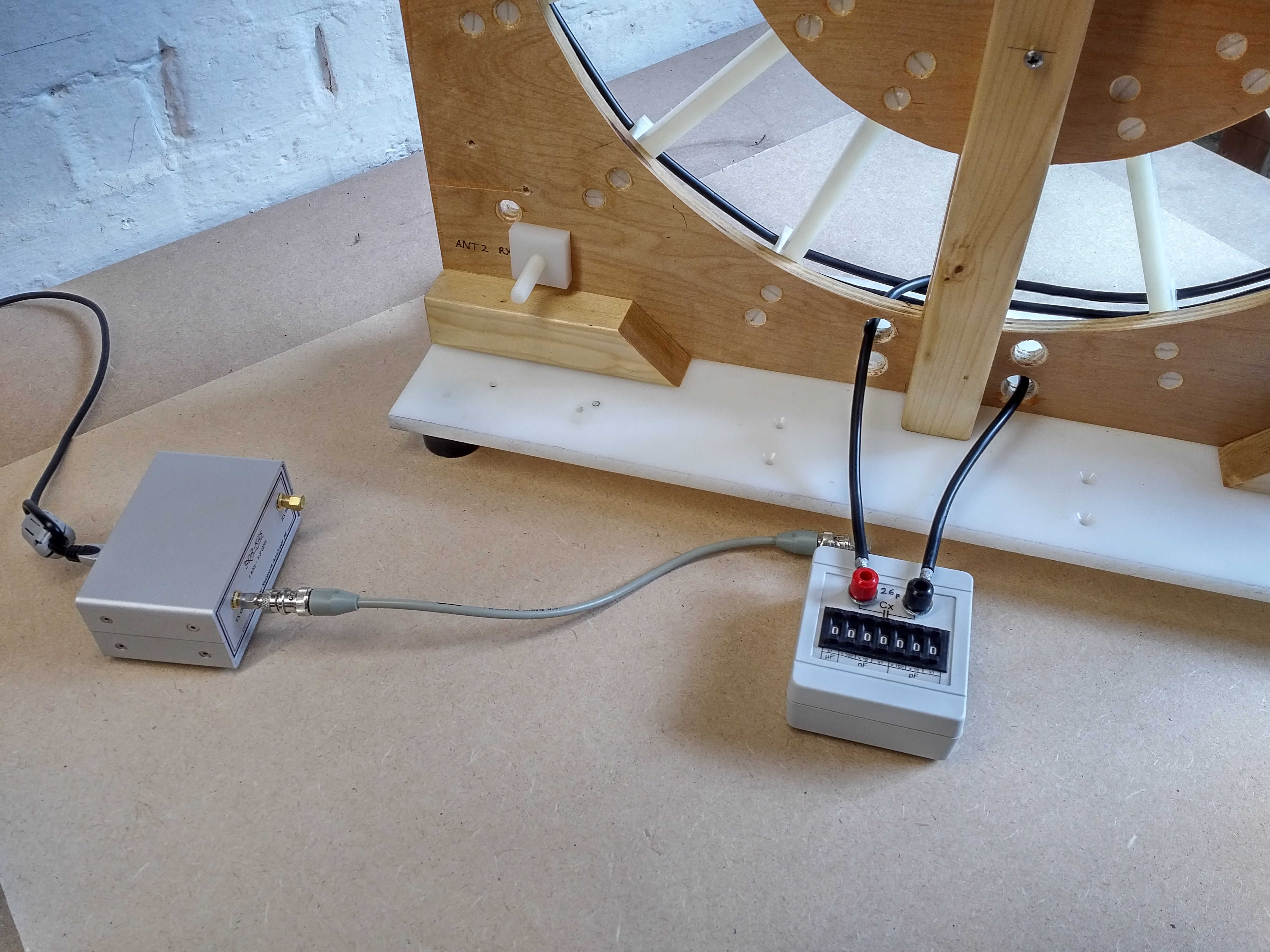
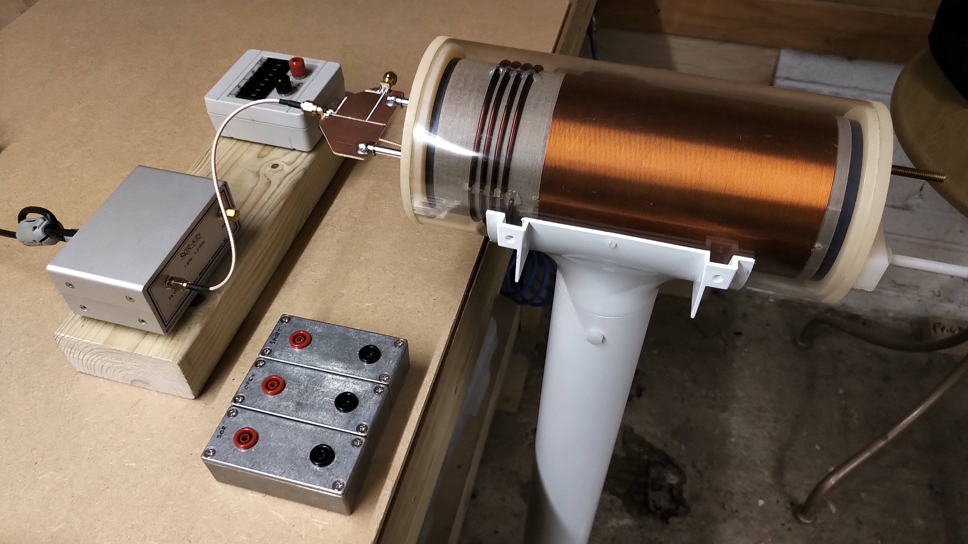
Fig. 1.4. Complete measurement circuit, calibrated VNA connected to the capacitance box which forms the tuning capacitance in parallel with the primary coil.
VNA-SDR Measurements for 1P Primary
Figures 2. show the wide frequency scan VNA impedance results for Z11 from calibration and through changing load capacitance on the primary. It is recommended to view the full-size scan images where the detail can be seen much clearer, (click on the image to see the full-size image and navigation icons). Below the figures 2. each individual result is considered and explained. In the explanations standard abbreviations are used as follows:
LP = Inductance of the primary coil.
CP = Capacitance box value connected in parallel with the primary coil.
LPCP = Parallel resonant circuit formed by the primary.
CPP = Self-capacitance of the primary including the parasitic capacitance of the capacitance box when set at 0pF, which in total has been measured to be 30.5pF.
FP = Fundamental resonant frequency of the primary.
LS = Inductance of the secondary coil.
CS = Self-capacitance of the secondary coil.
LSCS = Resonant circuit formed by the inductance of the secondary combined with self-capacitance of the secondary.
FS = Fundamental resonant frequency of the secondary (FS1).
FS2 = Second harmonic of FS up to FSN the nth-harmonic.
FØ = Frequency at which a phase change takes place.
FØ180 = Frequency at which a 180° phase change takes place.
FU = Upper resonant frequency of the flat coil.
FL = Lower resonant frequency of the flat coil.
M1 – MN = Frequency markers on the results can be identified with a down pointing arrow on the result curve with a number above it.
Q – The quality factor of an impedance feature. For example, as the Q increases a resonance peak will become sharper and narrower, and as the Q decreases a resonance peak will become more rounded and wider.
|Z| – Magnitude of the impedance, (|ZS| for secondary, |ZP| for primary, |ZU| for the upper frequency of the flat coil, and |ZL| for the lower frequency of the flat coil).
Ø – Phase of the impedance.
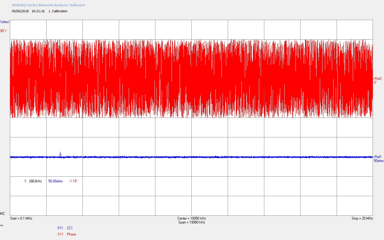
Fig. 2.1. Starting calibration over the range 0.1-20MHz using a standard 50Ω load
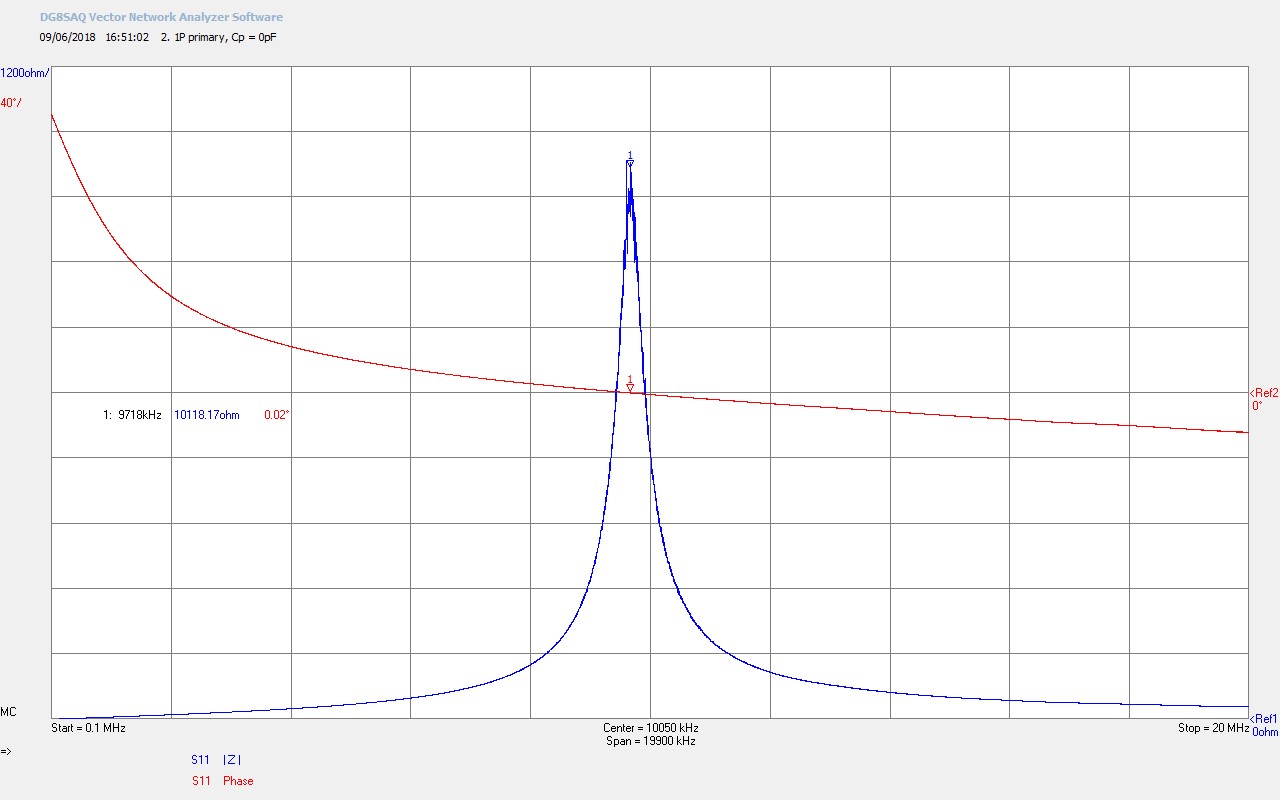
Fig. 2.2. 1P primary with load capacitance of Cp = 0pF (Parasitic capacitance Cpp = 30.5pF).
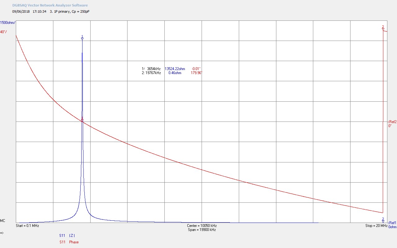
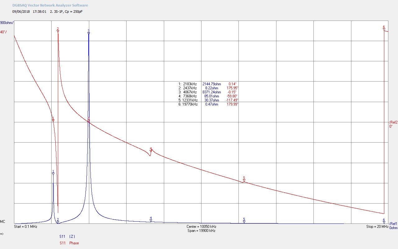
Fig. 2.3. 1P primary with load capacitance of Cp = 250pF.
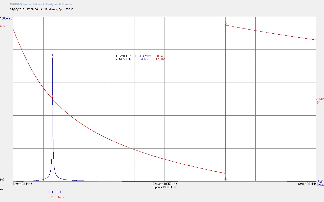
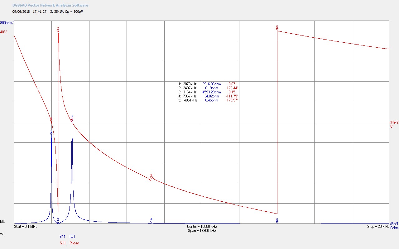
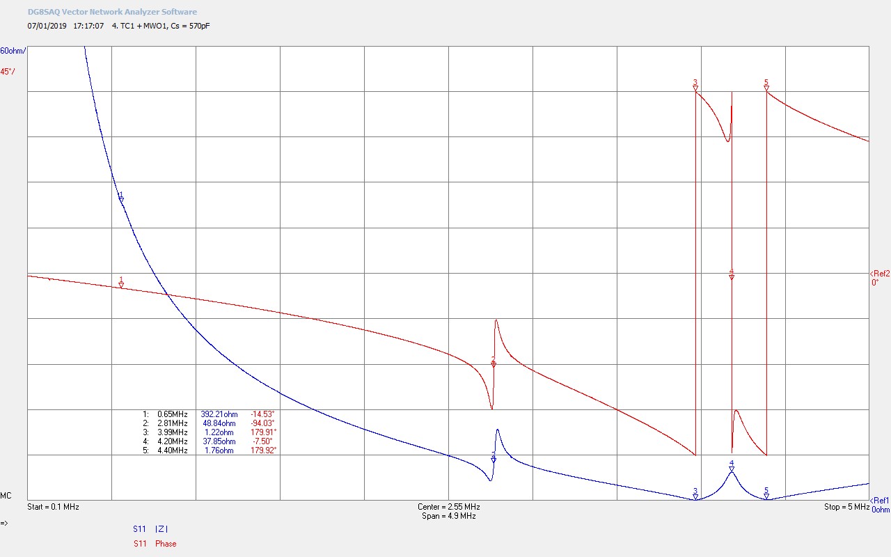
Fig. 2.4. 1P primary with load capacitance of Cp = 500pF.
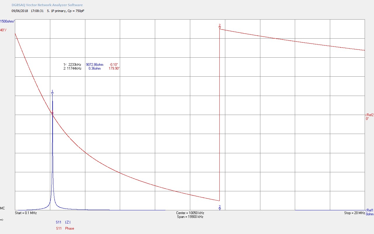
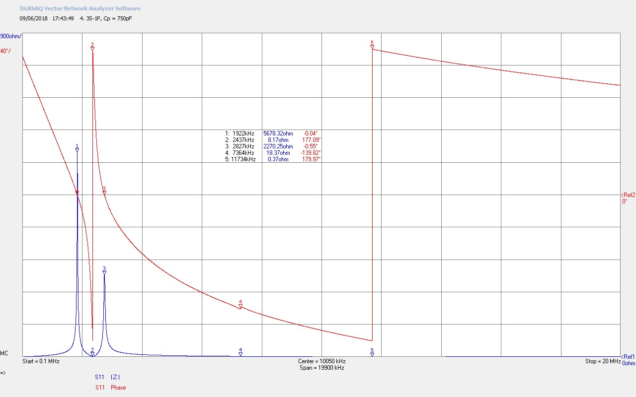
Fig. 2.5. 1P primary with load capacitance of Cp = 750pF.
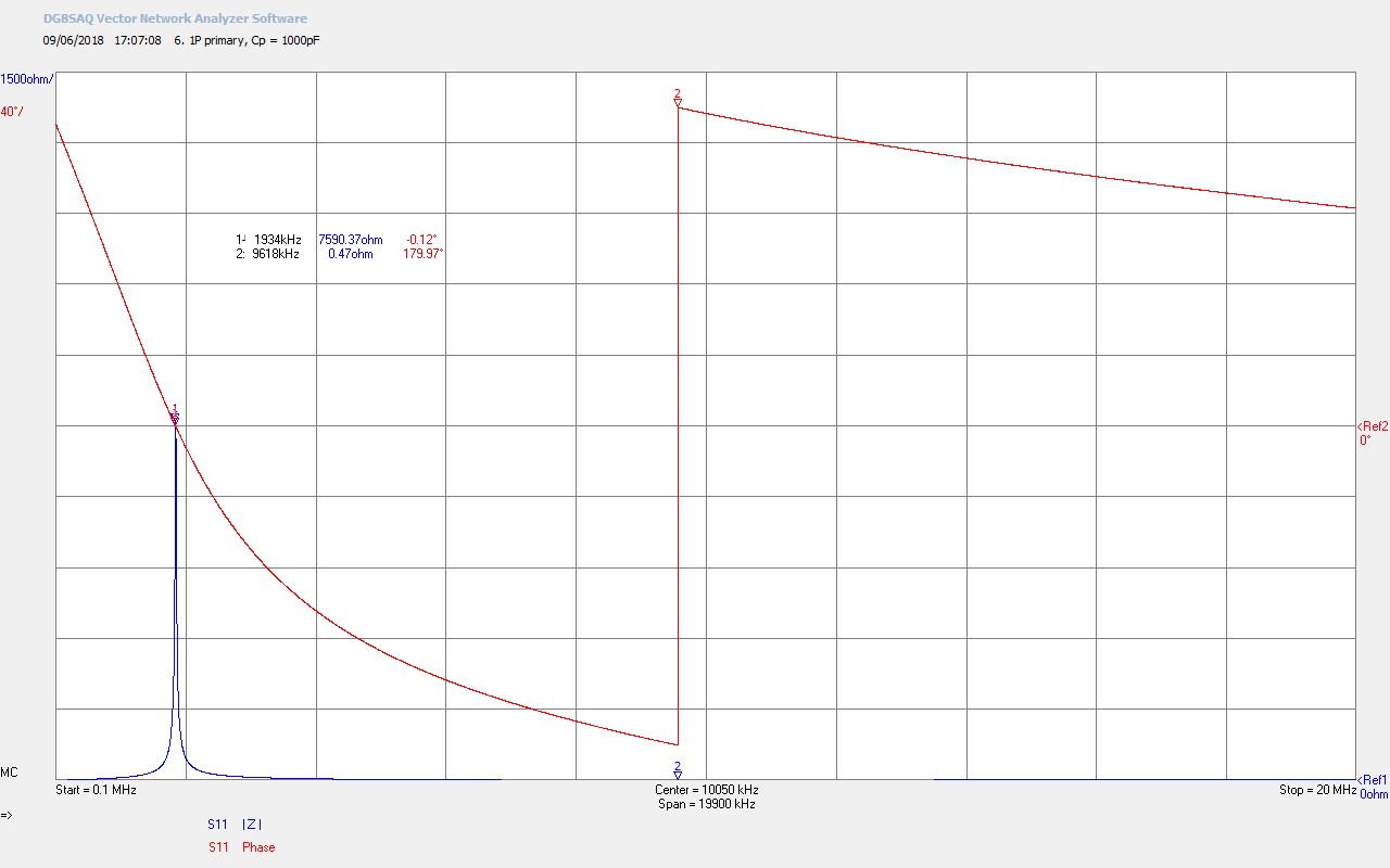
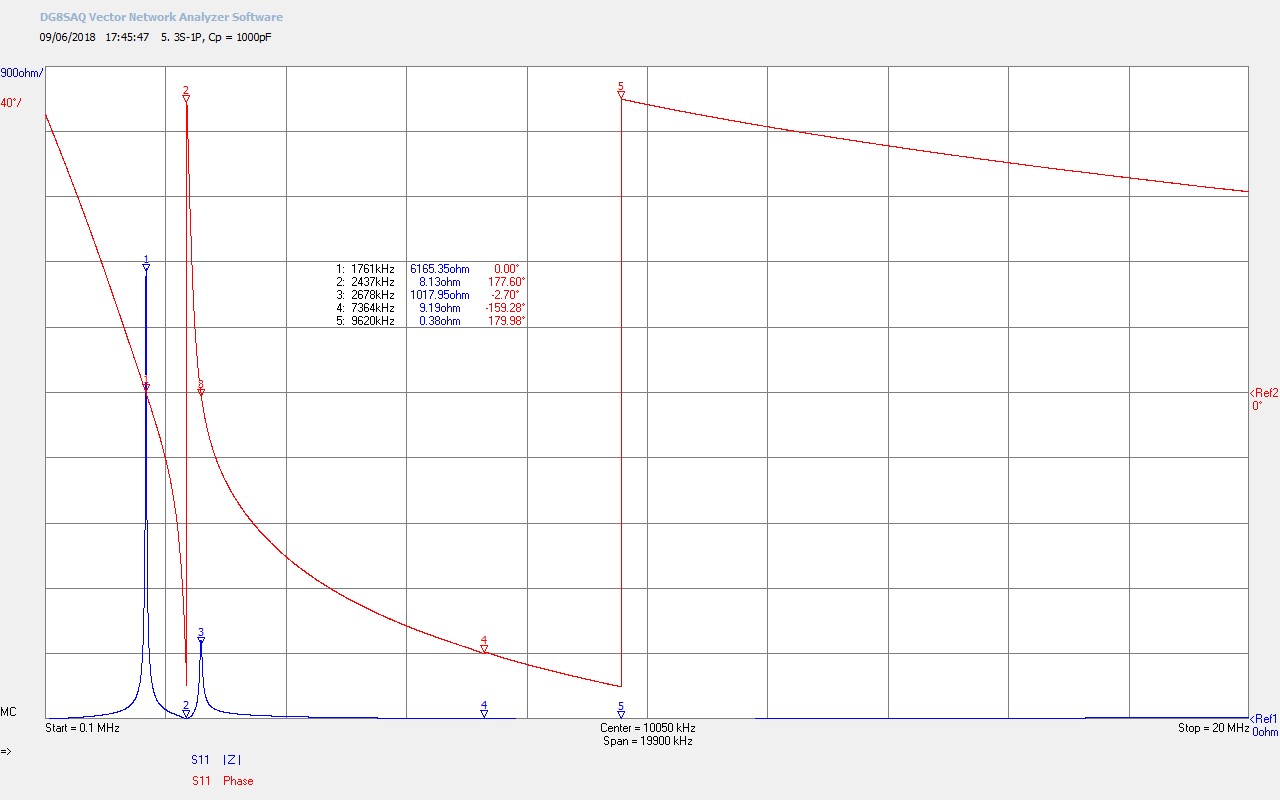
Fig. 2.6. 1P primary with load capacitance of Cp = 1000pF.
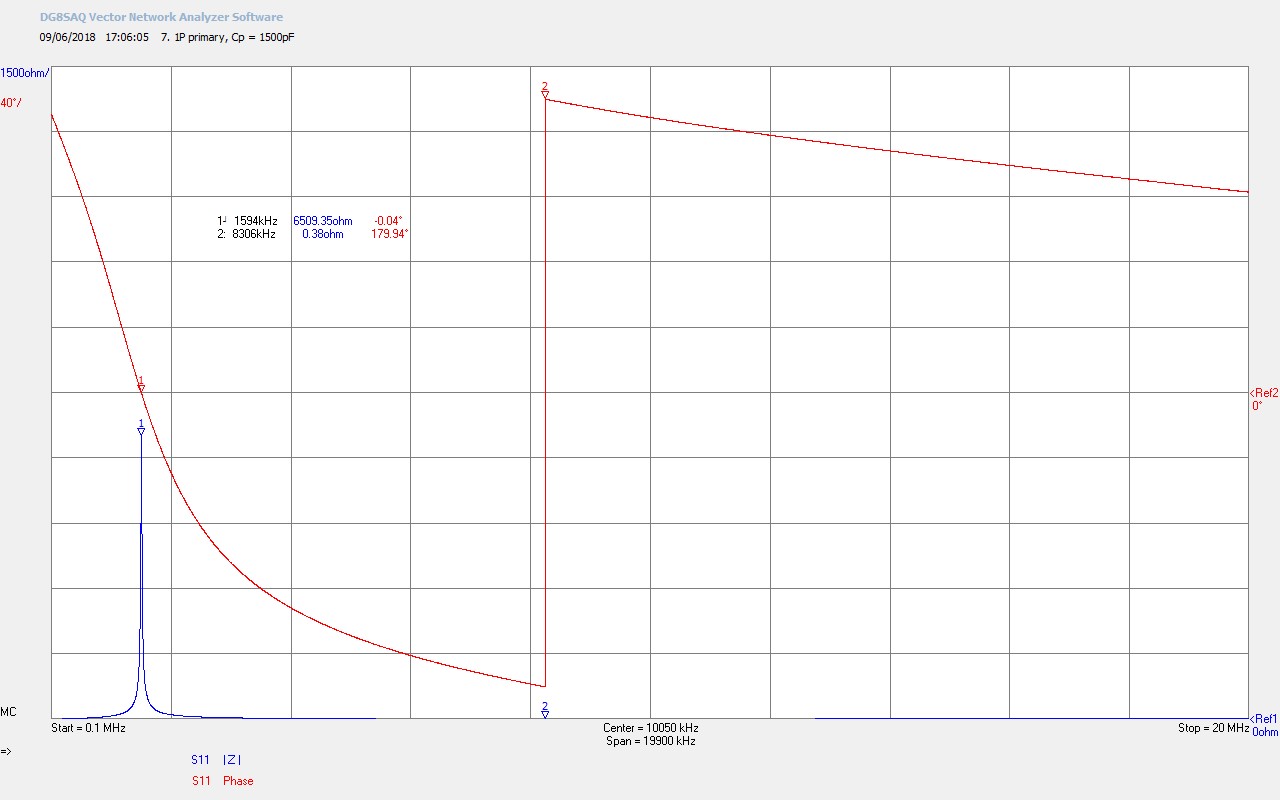
Fig. 2.7. 1P primary with load capacitance of Cp = 1500pF.
To view the large images in a new window whilst reading the explanations click on the figure numbers below:
Fig 2.1. Shows the calibration to the end of the bnc connected to the primary capacitance box (CP). For this calibration the bnc was terminated with a standard 50Ω load and can be seen to be constant over the calibrated range of 0.1Mc/s and 20Mc/s. The phase in the calibration will swing repeatedly between ±180° indicating the near perfect match between the output impedance of the VNA (50Ω) and the standard 50Ω termination, as expected for a calibration of this type of instrument. M1 confirms the impedance magnitude 50.00Ω and phase -1.19° at 2863kc/s.
Fig 2.2. Shows the 1P primary with CP=0pF (30.5pF from the self-capacitance of the primary turns and parasitic capacitance combined, CPP). There is a strong parallel self-resonance of the primary coil which results from combination LPCP. From marker M1 the fundamental resonant frequency FP=9718kc/s with the 180° phase change, characteristic of a resonant circuit, shifted to a much higher frequency above the upper limit of the scan (20Mc/s). The large shift between FØ180 and FP results from the large imbalance between the inductance of the coil LP and the very small self-capacitance CP . As CP starts to rise in the following figures FØ180 will start to fall in frequency.
Fig 2.3. Shows the effect of increasing CP=250pF. FP has now dropped considerably to 3654kc/s and FØ180 has just entered at the far end of the scan at 19767kc/s. The magnitude of the impedance has increased as the resonance has strengthened, and the Q of the coil has also increased as lumped element capacitance stabilises the electrical properties of the circuit and dominates over the self-capacitance of the coil.
Fig 2.4. Increasing CP=500pF continues to reduce FP and FØ180. The magnitude of the impedance |Z| continues to fall and the Q reduces slightly.
Fig 2.5. Increasing CP=750pF continues to reduce FP and FØ180. |Z| continues to fall as the parallel resonance weakens, and FP passes through what will be FØ180 of the secondary coil when added to the primary.
Fig 2.6. Increasing CP=1000pF continues to reduce FP and FØ180. |Z| continues to fall, and FP comes into the fundamental band of operation (1810-2000kc/s).
Fig 2.7. Increasing CP=1500pF continues to reduce FP and FØ180. |Z| continues to fall, and FP goes below the fundamental band of operation and into the medium wave (MW) band.
Overall the effect of increasing the primary capacitance CP is to progressively reduce the primary’s fundamental resonant frequency FP. As a better balance between LPCP is established the wide gap between FP and FØ180 reduces. FP appears to go through an optimal point of resonance where the impedance |Z| is maximum and the Q is maximum at a resonant frequency FP ~ 4500kc/s and CP ~ 195pF. The shifting of FP with CP will allow the complete flat coil 3S-1P to be tuned, as the resonant circuit in the primary interacts with the resonant circuit in the secondary. These two coupled resonant circuits form the overall impedance characteristics of the flat coil as investigated below. No harmonics of the fundamental where observed in the impedance scans of the primary.
VNA-SDR Measurements for 3S-1P
Figures 3. show the wide frequency scan VNA impedance results for Z11 with changing load capacitance on the primary.
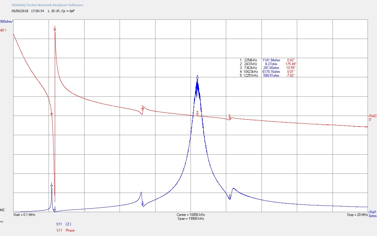
Fig. 3.1. 3S-1P, Cp = 0pF.
Fig. 3.2. 3S-1P, Cp = 250pF.
Fig. 3.3. 3S-1P, Cp = 500pF.
Fig. 3.4. 3S-1P, Cp = 750pF.
Fig. 3.5. 3S-1P, Cp = 1000pF.
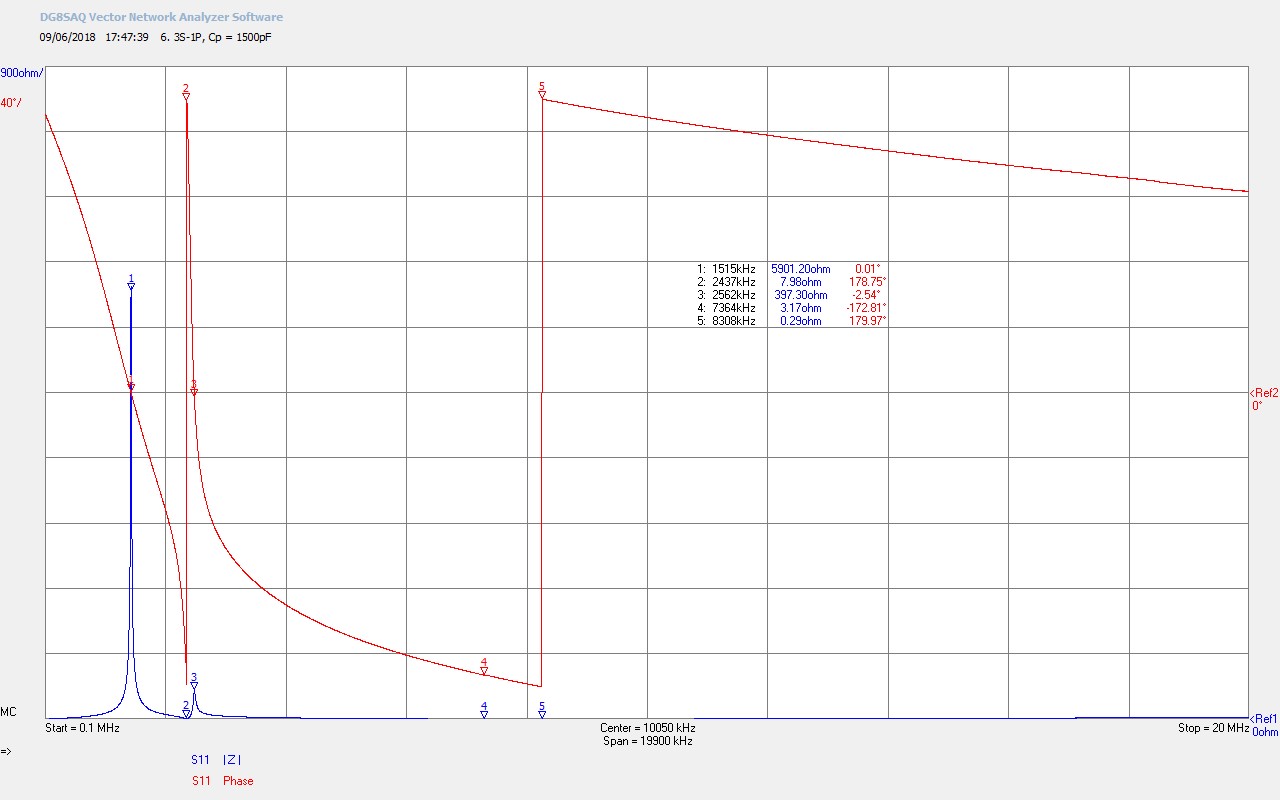
Fig. 3.6. 3S-1P, Cp = 1500pF.
To view the large images in a new window whilst reading the explanations click on the figure numbers below:
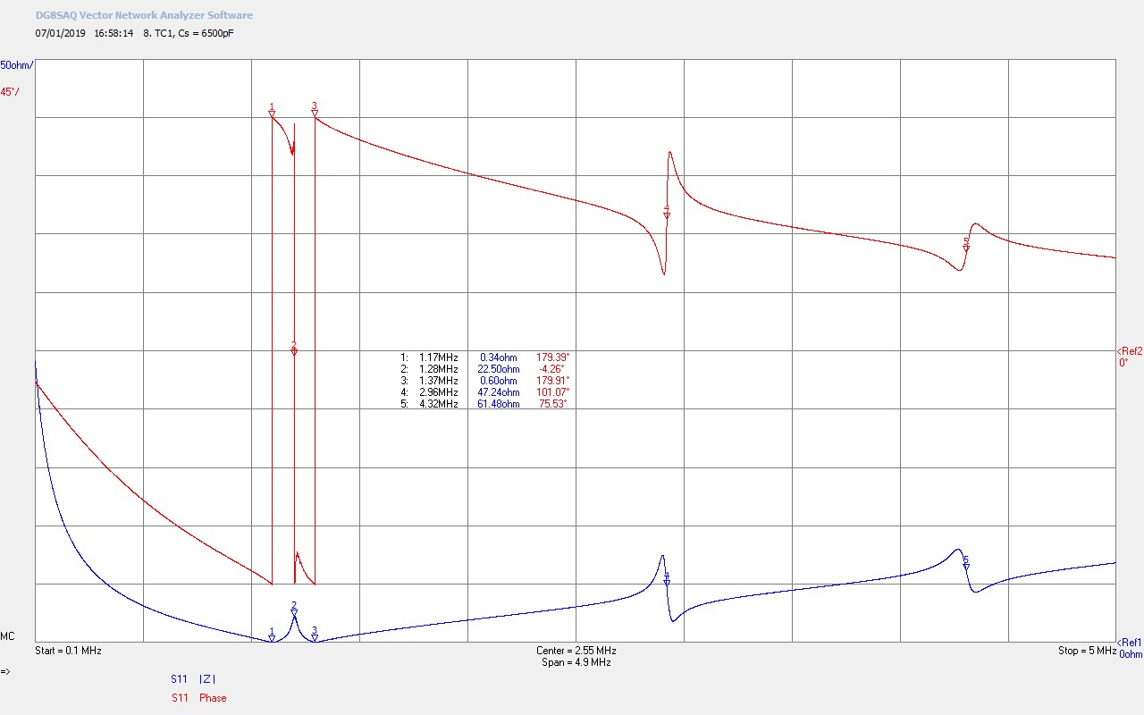
Fig 3.1. Shows the secondary and the primary combined together in frequency and with CP = 0pF. Here the two resonant characteristics appear superimposed on one another. The self-resonance of the primary is very clearly defined at M4, and is very similar to that measured in the primary only results of Fig 2.2. The self-resonance of the secondary has generated the fundamental FS = 2254kc/s at M1 and FØ180 = 2437kc/s at M2. For the secondary FØ180 is defined by the effective wire length used in λ/4 mode with the addition of an impedance lowering extension at the bottom-end of the coil. In Part 1 of the design the wire length was to be arranged to give FØ180 = 2400kc/s which is very close to the result measured. The fundamental operating frequency was designed to fall into the 160m amateur band (1810-2000kc/s), and currently FS = 2254kc/s slightly above this band. In operation CP in the primary will be adjusted in order to tune the resonant operating frequency into the required band. The balance between LSCS is much better in the secondary as the self-capacitance of the many turns is much bigger and more stable than that for the primary, and so the gap between FP and FØ180 is smaller, and in this case also contributed to by the series resistance of the secondary coil. Q appears reasonable at this stage and the impedance |Z| is much lower than that for the primary which most likely results from the inter-winding capacitive network of the secondary. There are 2 odd harmonics above the fundamental FS2 at M3 and FS3 at M5 which occur at 3λ/4 and 5λ/4 respectively. It maybe by chance but it is interesting to note that FP is not that far away from 4λ/4 for the secondary. Whether this will have any impact on the performance of the flat coil remains to be established.
Fig 3.2. Increasing CP = 250pF has mainly, and as expected from figures 1, reduced the primary resonant frequency FP down to a frequency much closer to the secondary. Here we can see the start of the formation of the flat coil upper and lower resonant frequencies. The FØ180 point at M2 stays constant as the effective wire length of the secondary is not changing and dominates the fundamental FS of the secondary. The lower frequency FS at M1 from the secondary forms the lower frequency of the flat coil, and starts to move away from FØ180as CP is increased, which allows tuning of FS to the required frequency using CP. The upper frequency FP at M3 from the primary forms the upper frequency of the flat coil, and moves progressively down towards FØ180as CP is increased. As two coupled circuits cannot resonate at exactly the same frequency when CP is continued to be increased > 1000pF FS and FP will appear to swap position, with FP emerging below FS and whilst close to FS appearing to push FS slightly above FØ180. When two or more coupled resonant circuits interact the energy exchange between the modes of vibration creates beating and a particular mode becomes dominant (drives) coupling energy from one resonant circuit to the other. It is in this region that the flat coil is most interesting to investigate, and an important factor in the study of the displacement and transference of electric power. These coupled modes of FP and FS will be investigated in more detail on Figures 4., and practically within the experiments.
Fig 3.3. Increasing CP=500pF starts to bring the upper and lower frequencies of the flat coil into closer balance. |ZS| at M1 is increasing in impedance as the parallel resonance in the secondary is strengthened by coupling from the primary, whilst |ZP| at M3 is reducing. The overall effect is to bring the electric and magnetic fields of induction, across the primary and the secondary, towards a more balanced point. It is this point of balance (harmony between the two induction fields) that is conjectured to be the optimal point to trigger a non-linear event. It is conjectured that a non-linear event at this point of balance, and dependent on the form of the load connected, will generate a coherent displacement event between the generator (source) and the load(s). This consideration will be developed further during the experimental reporting, and in conjunction with actual results obtained.
Fig 3.4. Increasing CP=750pF has now passed through the balance point between the fields of induction and to where the lower frequency starts to dominate the resonance of the flat coil, and the upper frequency will now continue to diminish. The lower frequency FS at M1 is now within the 160m of operation. FØ180 remains unchanged. Harmonics are diminishing as the resonance of the secondary starts to be suppressed by the high capacitive loading of the primary.
Fig 3.5. Increasing CP=1000pF the primary resonance FP is dominating the overall resonance at the lower frequency of the flat coil. Secondary coil harmonics have almost completely been suppressed by the high capacitive loading of CP. The lower resonant frequency at M1 has now moved out of the lower end of the 160m amateur band.
Fig 3.6. Increasing CP=1500pF the primary resonance FP is now totally dominating the overall resonance at the lower frequency of the flat coil. The lower resonant frequency at M1 has now moved into the medium wave band at 1515kc/s.
When CP is lower, and in the range ~200 – 450pF, the overall resonance of the flat coil is dominated by FP the fundamental resonant frequency of the primary, and what has formed the upper resonant frequency of the flat coil ~ 2700kc/s – 4500kc/s. When CP is larger, and >950pF, the overall resonance of the flat coil is again dominated by FP the fundamental resonant frequency of the primary at the lower resonant frequency of the flat coil < 1750kc/s. In between, in the range 450pF < CP < 950pF, there is a more established balance between FS and FP and the upper and lower resonant frequencies of the flat coil are determined by the interaction and energetic exchange between the secondary and the primary. It is this region that is most interesting to experiments in the displacement and transference of electric power, and whose impedance characteristics are investigated in more detail below.
Figures 4. show the narrow frequency scan VNA impedance results for Z11 at a key set of different load capacitance.
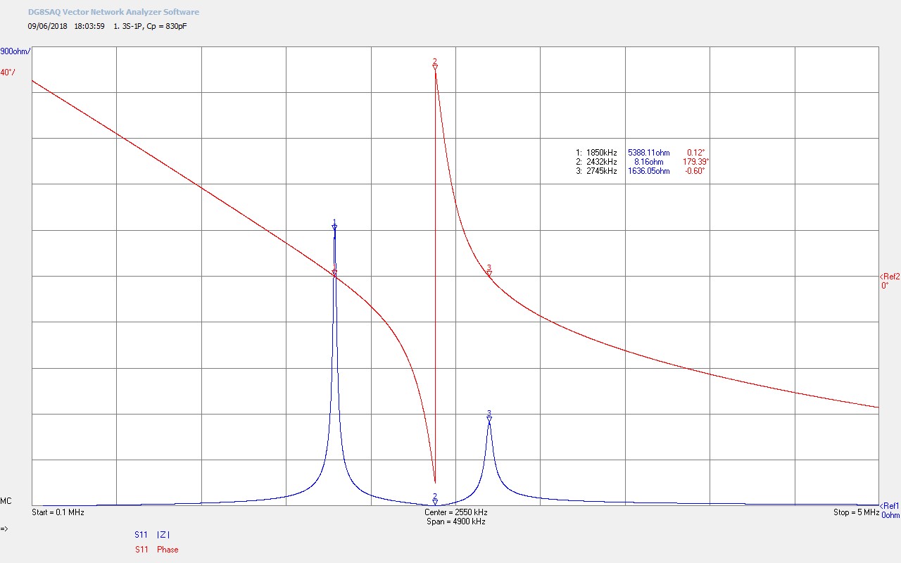
Fig. 4.1. 3S-1P tuned to a fundamental resonant frequency of 1.85MHz, Cp = 830pF.
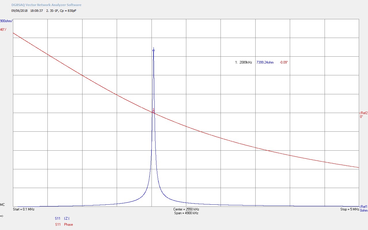
Fig. 4.2. 1P only when 3S-1P was tuned to the fundamental resonant frequency of 1.85MHz, Cp = 830pF.
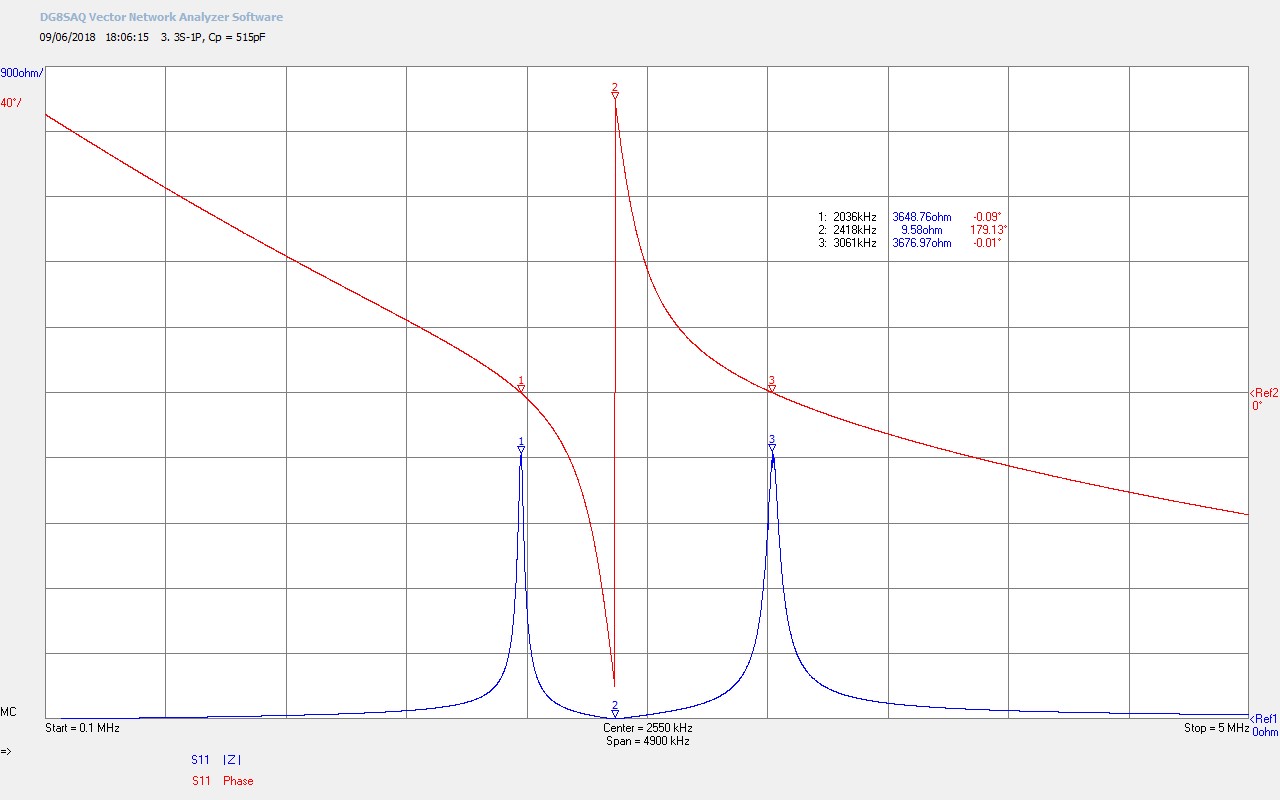
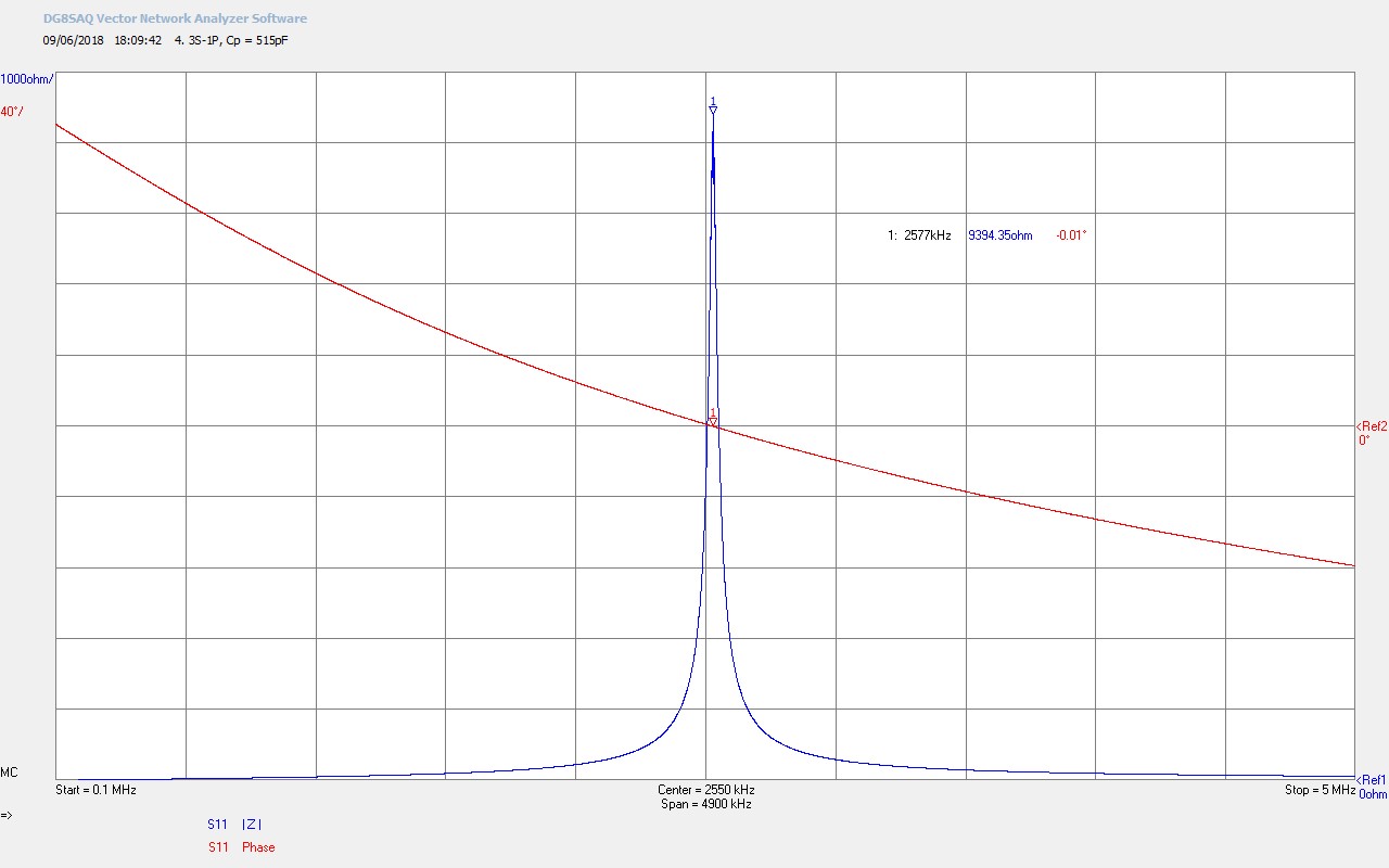
Fig. 4.3. 3S-1P tuned so that resonant frequencies at markers 1 and 3 have an equal impedance magnitude, Cp = 515pF.
Fig. 4.4. 1P only when 3S-1P was tuned so that resonant frequencies at markers 1 and 3 have an equal impedance magnitude, Cp = 515pF.
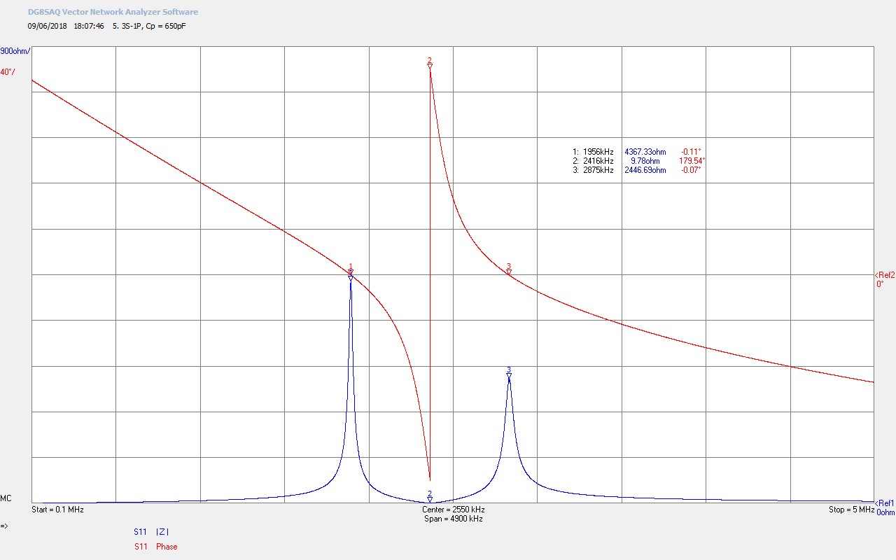
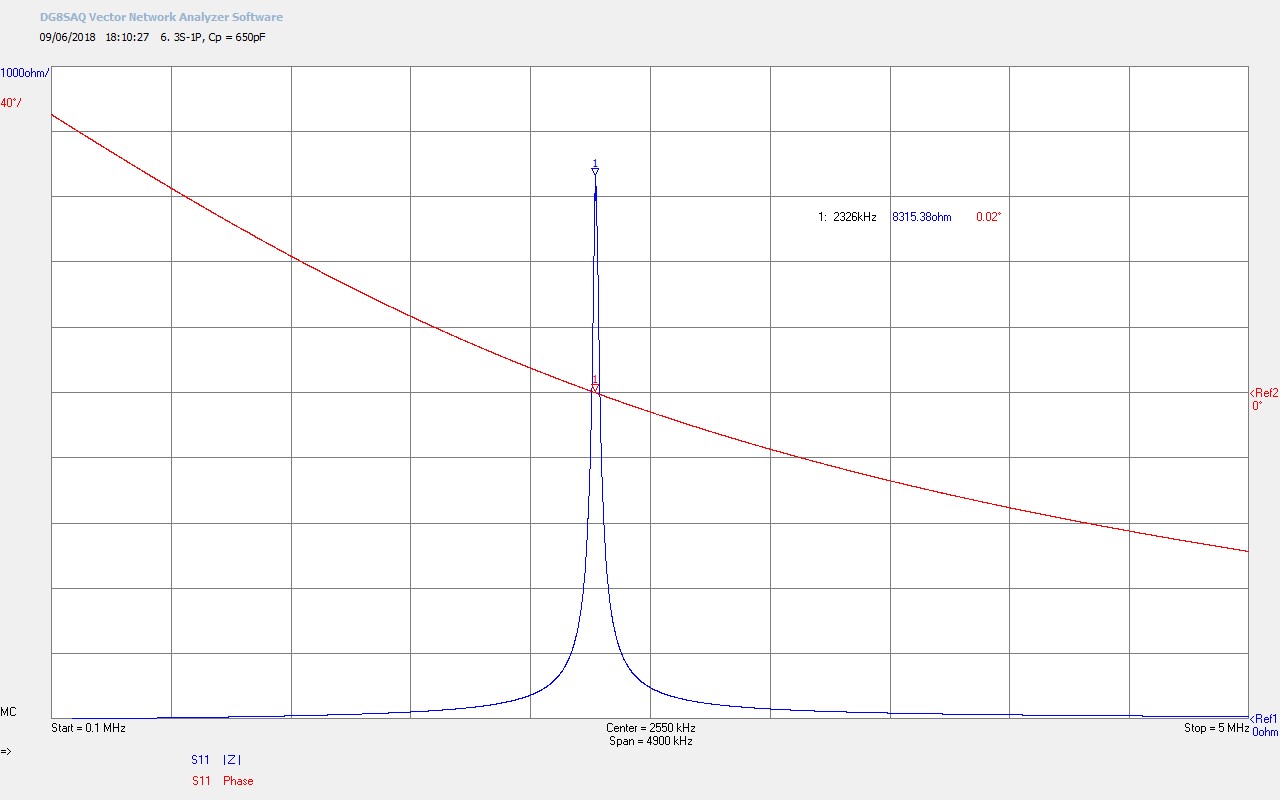
Fig. 4.5. 3S-1P tuned to a point where the resonant frequencies at markers 1 and 3 are equidistant in frequency from the 180° at marker 2, Cp = 650pF.
Fig. 4.6. 1P only when 3S-1P was tuned to a point where the resonant frequencies at markers 1 and 3 are equidistant in frequency from the 180° at marker 2, Cp = 650pF.
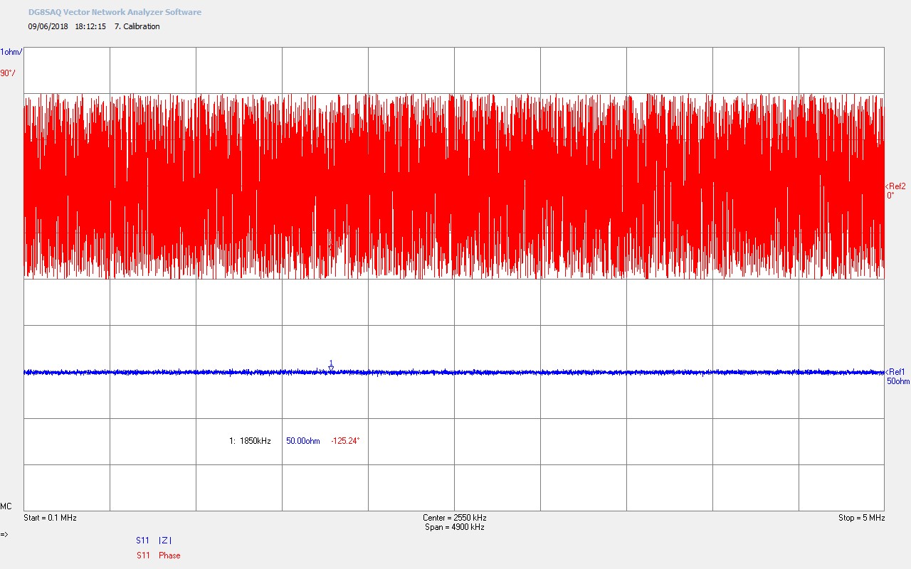
Fig. 4.7. Ending calibration over the range 0.1-5MHz using a standard 50Ω load.
To view the large images in a new window whilst reading the explanations click on the figure numbers below:
Fig 4.1. Here the primary capacitance CP = 830pF has been adjusted so that the lower resonant frequency of the flat coil FL at M1 is at the nominal designed point of 1850kc/s in the 160m amateur band. When setup to self-resonate with feedback from the flat coil to the generator the flat coil will stably oscillate at FL, and will form a base starting point for the experiments in the displacement and transference of electric power.
Fig 4.2. Shows the resonant frequency of the primary FP when the secondary is removed from the flat coil, and all other conditions and setup are kept the same. FP is closer to the lower resonant frequency of the flat coil FL than the upper FU, which corresponds with a stronger resonance at FL, and a weaker one at FU, and hence |ZL| > |ZU|.
Fig 4.3. Here the primary capacitance CP = 515pF has been adjusted so that the magnitude of the impedance at the upper resonant frequency is equal to the magnitude of the impedance at the lower resonant frequency |ZU| = |ZL|. It is conjectured that at this point there is balanced interaction between the secondary and primary resonance points which is optimal for the balanced energetic inter-exchange between the electric and magnetic fields of induction between the two coils. It is at this point where best coherence between the two fields of induction can be established, and hence a significant pre-condition to displacement established. It is also conjectured that the initiation of a displacement event requires a non-linear trigger within the system being tested whether that originates from the generator, the coils, or is stimulated as a response (pulled by) the load. It is the purpose of the experimental measurements to establish if this or another mechanism is the case, and the properties and characteristics under which they occur.
Fig 4.4. Again shows the resonant frequency of the primary FP when the secondary is removed from the flat coil, and all other conditions and setup are kept the same. Here we can see that FP at M1 (2577kc/s) occurs almost exactly equi-distant between FS and FP with the secondary added to the flat coil. From Fig. 4.1. (FP – FS) / 2 + FS = 2548.5kc/s, and from Fig. 4.2. FP = 2577kc/s (<2% difference). Here the resonance of the primary FP has inter-acted with the resonance of the FS so that both contribute equally to the overall flat-coil characteristic and hence establishing the balance between the electric and magnetic fields of induction as discussed in Fig. 4.1.
Fig 4.5. Here the primary capacitance CP = 650pF has been adjusted so that the upper FU and lower FL resonant frequencies of the flat-coil are equi-distant from the 180° phase change frequency of the secondary, FØ180. The resonant frequency of the secondary FS (FL) has just moved into the 160m amateur band at 1956kc/s, and |ZS| wil start to dominate the resonance of the flat coil. When allowed to self-resonate with feedback to the generator the flat coil will stably oscillate at FS.
Fig 4.6. Again shows the resonant frequency of the primary FP when the secondary is removed from the flat coil, and all other conditions and setup are kept the same. FP has progressed down slightly in frequency with increased CP from Fig. 4.4. as expected.
Fig 4.7. Calibration test at the end of the measurement period using a standard 50Ω load, with M1 confirming 50Ω at 1850kc/s.
VNA-HP Measurements for 3S-1P
Figures 5. show a selection of frequency results to confirm and check the accuracy of the results from two different VNAs, and also a basic equivalent circuit analysis for the primary S3 the narrow frequency scan VNA impedance results for Z11 at a key set of different load capacitance.
Fig. 5.1. 1P primary with load capacitance of Cp = 0pF (Parasitic capacitance Cpp = 30.5pF).
Fig. 5.2. 1P primary with load capacitance of Cp = 750pF.
Fig. 5.3. Equivalent circuit model of the 1P primary with load capacitance of Cp = 750pF.
Fig. 5.4. 3S-1P, Cp = 0pF.
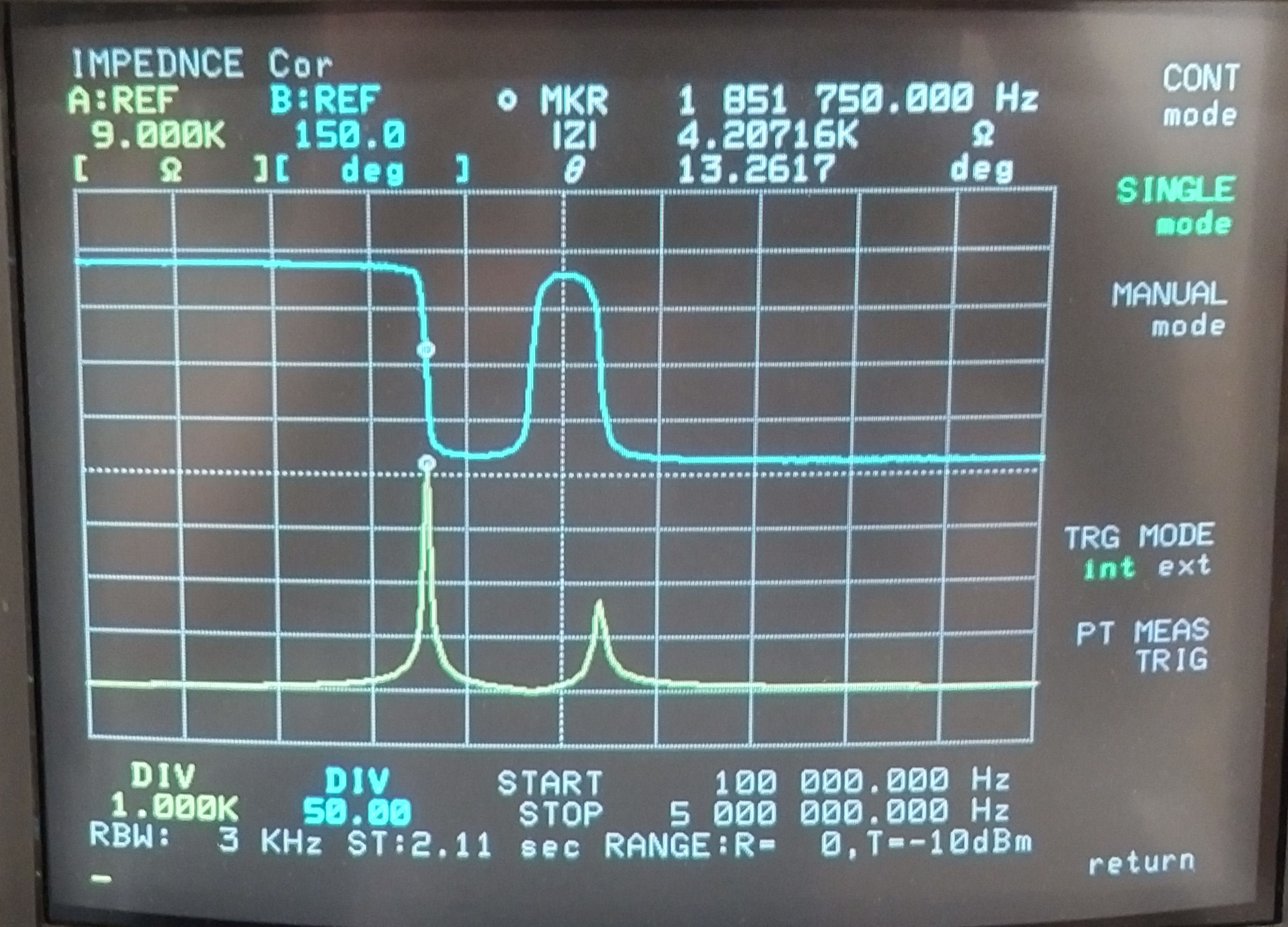
Fig. 5.5. 3S-1P tuned to a lower fundamental resonant frequency of 1.85MHz, Cp = 830pF.
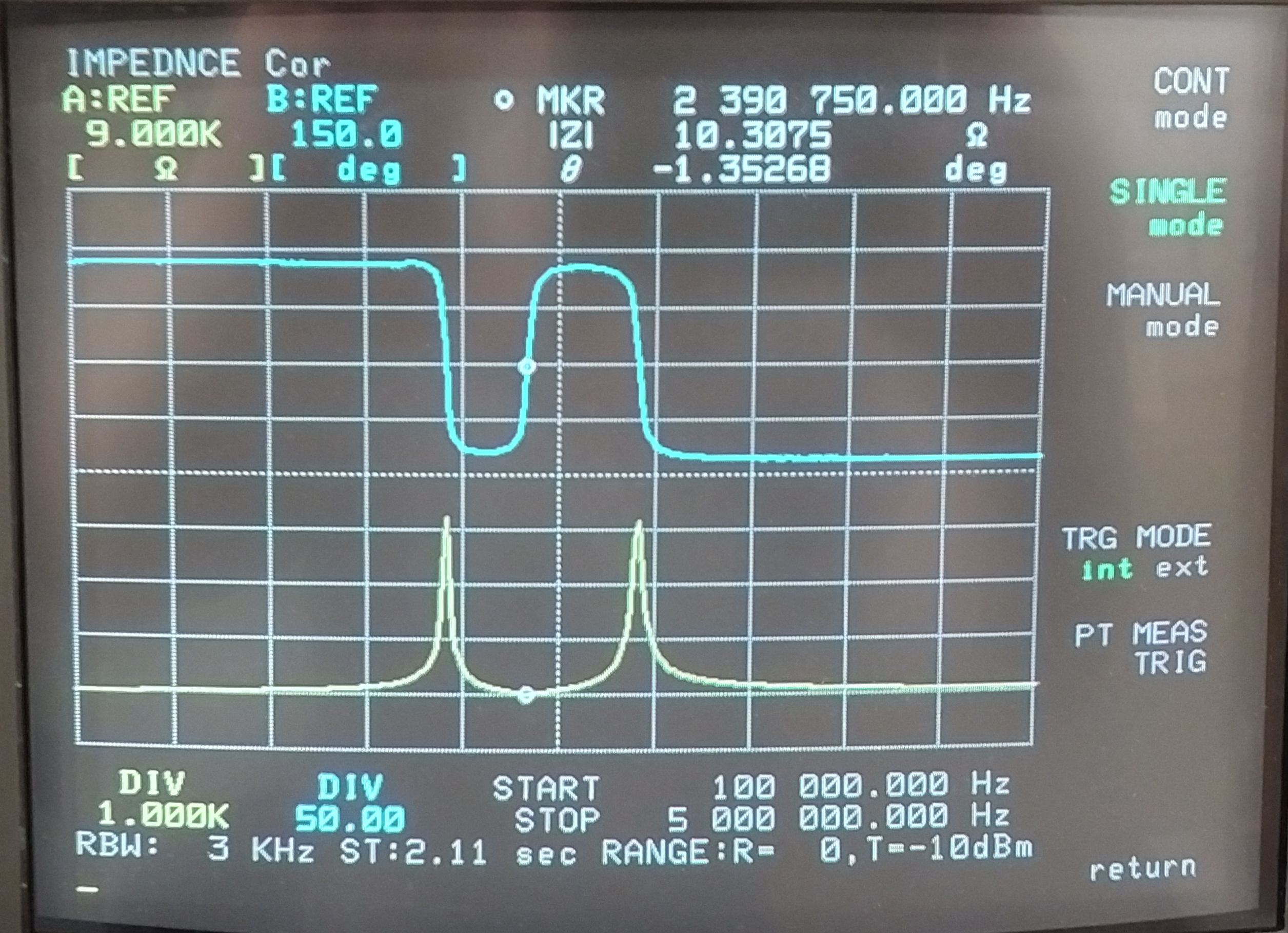
Fig. 5.6. 3S-1P tuned so that the upper and lower resonant frequencies have an equal impedance magnitude, Cp = 515pF.
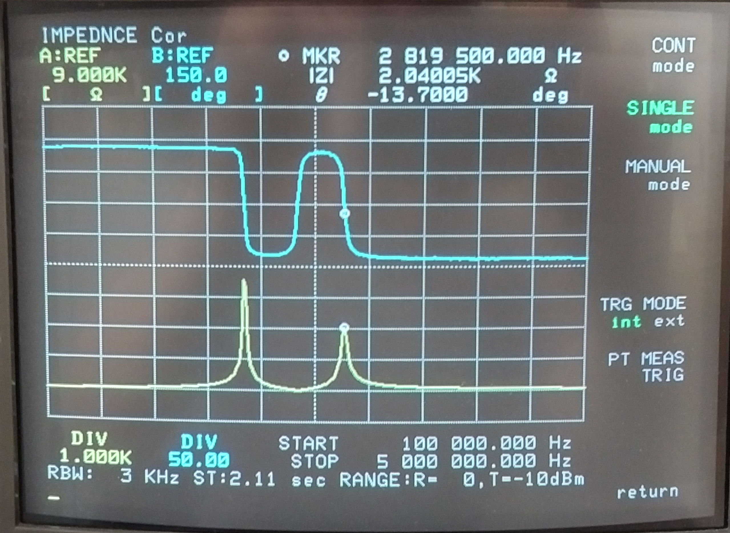
Fig. 5.7. 3S-1P tuned to a point where the uppoer and lower resonant frequencies are equidistant in frequency from the 180° phase change, Cp = 650pF.
To view the large images in a new window whilst reading the explanations click on the figure numbers below:
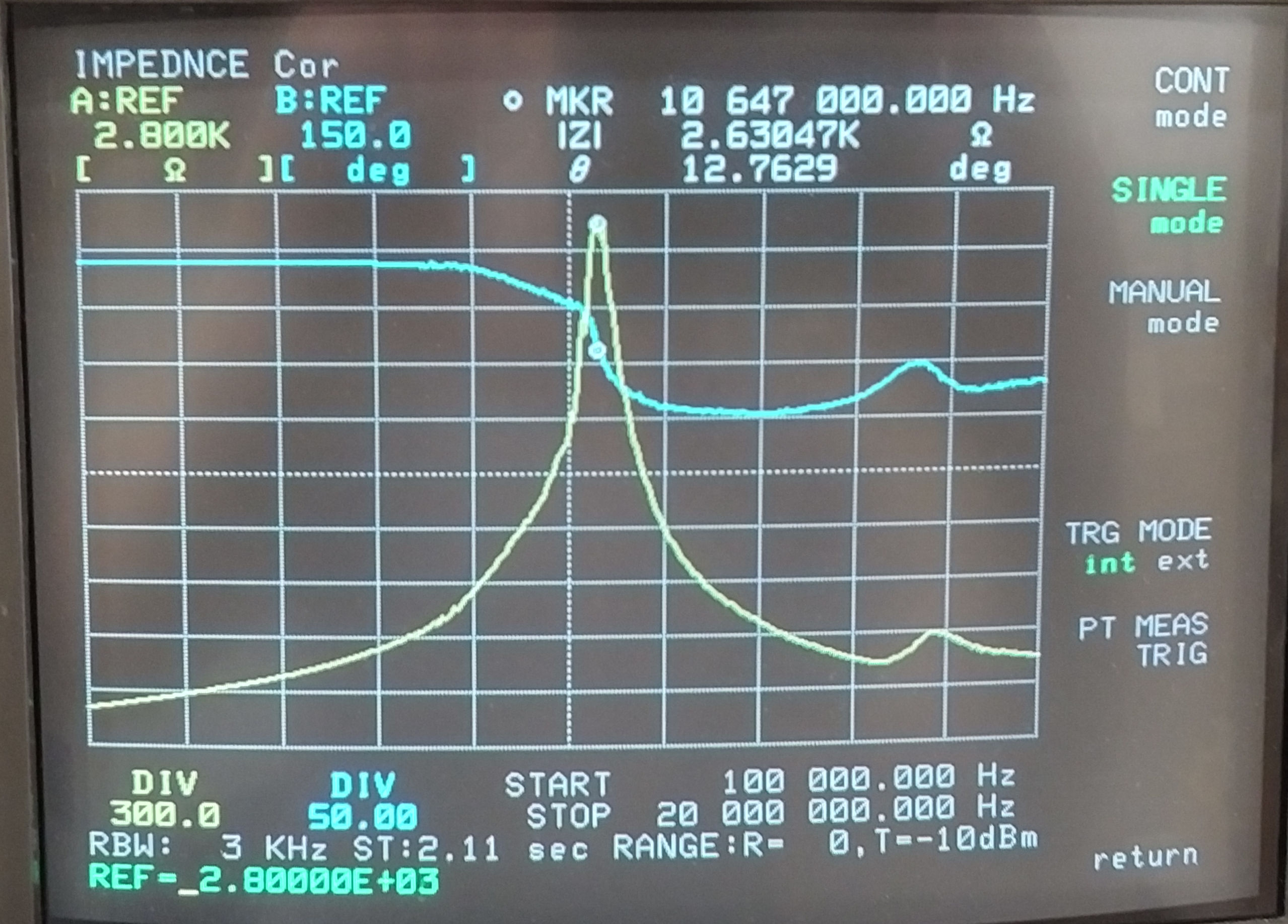
Fig 5.1. Shows the 1P primary with CP=0pF as per the measurement of Fig. 2.2. FP at the MKR frequency is 10647kc/s as measured by the VNA-HP, and was previously measured as 9718kc/s as measured by the VNA-SDR which represents ~ 9% variation in this measurements between the two methods. The phase curve indicated by the VNA-HP also shows a large variation corresponding to FP indicating the fundamental resonant frequency of the primary, and some further small impedance variation and phase change at ~18Mc/s. This highlights the difficulty of making measurements directly on the primary where there is a large imbalance between LP and CP which easily leads to varying measurement conditions easily influenced by the surrounding factors such as earthing structures, conductors, and other electrical loading influences. As LP and CP come into better balance this stabalises and a much greater measurement accuracy is obtained between both measurement machines.
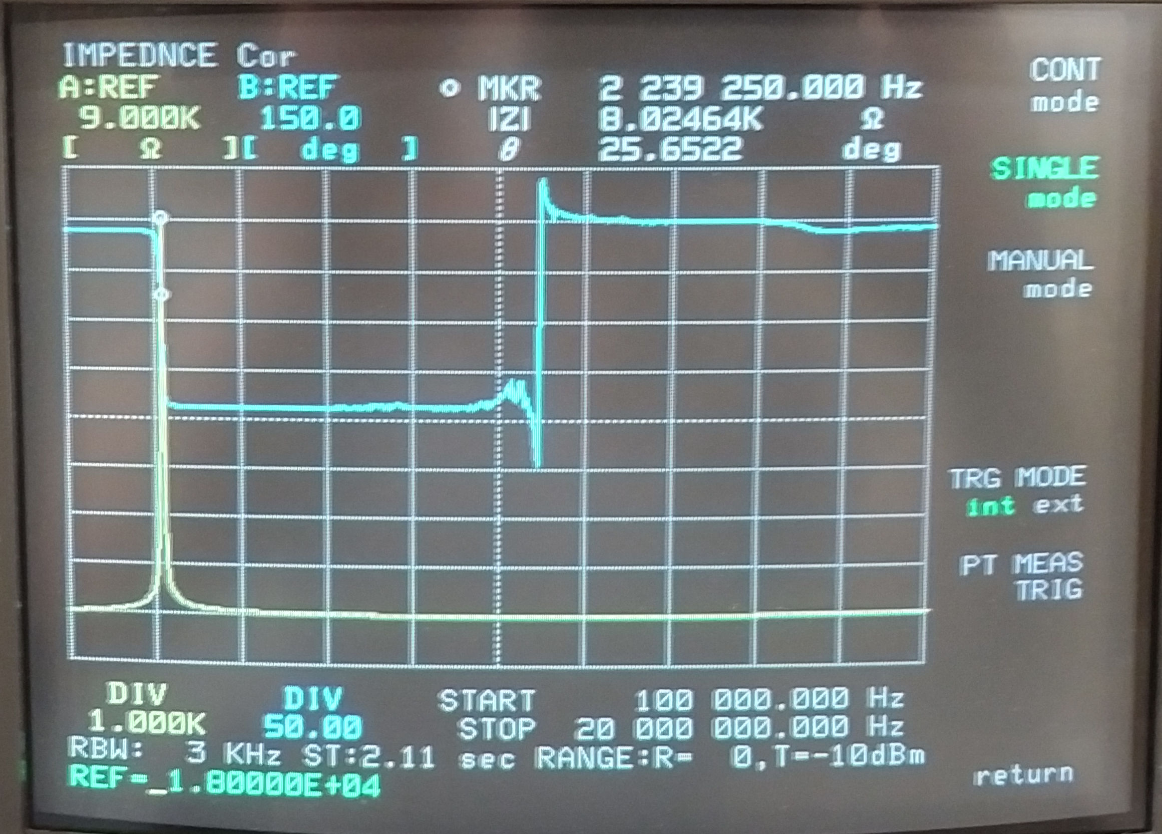
Fig 5.2. Increasing CP=750pF as per the measurement in Fig., 2.5. the 1P primary resonant frequency has moved to 2239.25kc/s, and was previously measured as 2233kc/s by the VNA-SDR showing < 0.5% variation in the frequency. |Z| measures as 8.02kΩ, and was previously 9.072kΩ showing ~12% variation. FØ180 measures as 11000kc/s and was previously 11744kc/s ~7% variation.
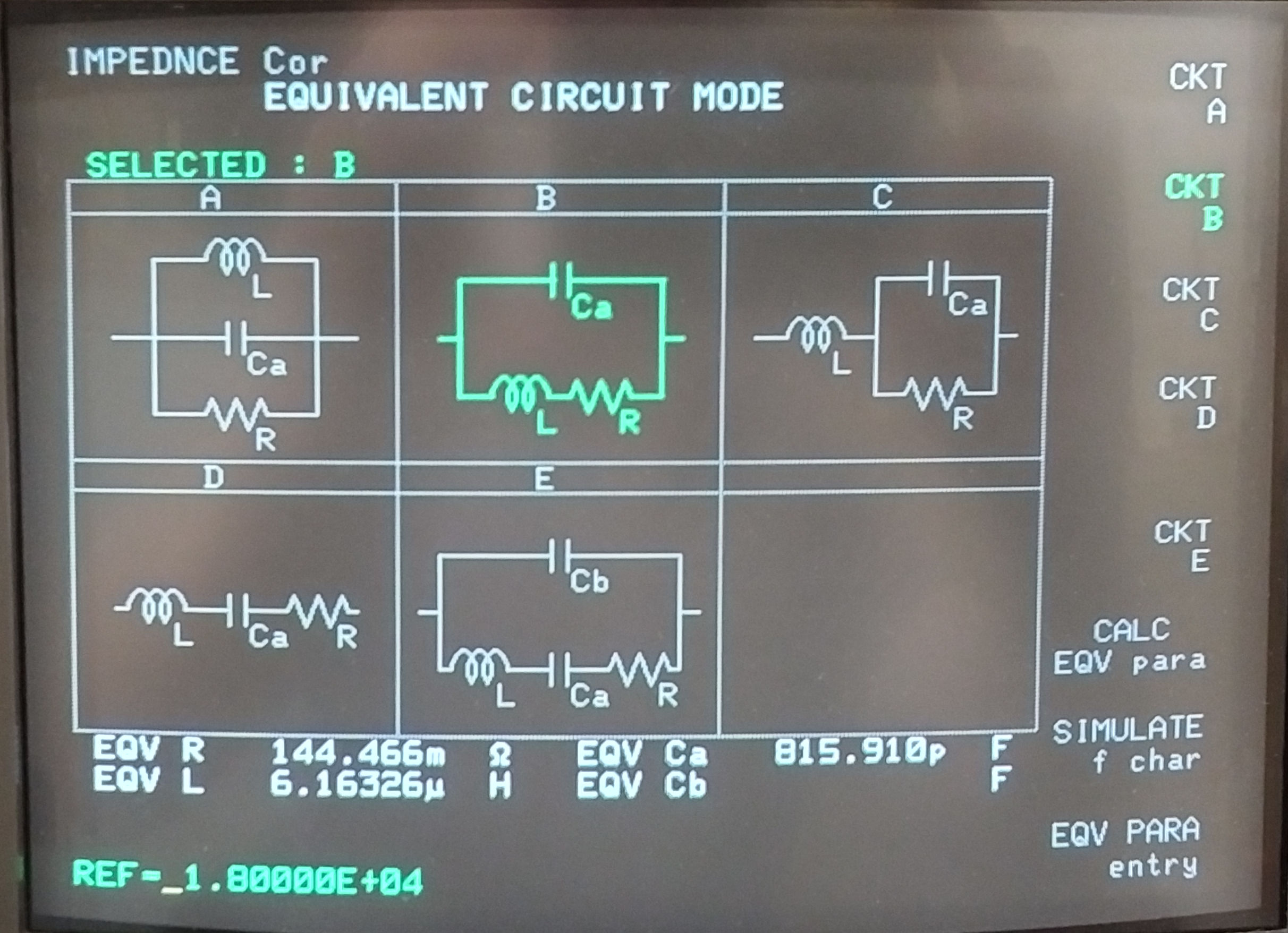
Fig 5.3. Shows the computed equivalent circuit of the 1P primary conditions as per Fig. 5.2. The equivalent circuit is calculated by the HP4195A based on a fit model to the measured curve. In part 1 of the impedance measurements the inductance of the 1P primary was measured at 6.453µH, and here is modelled as 6.163µH ~5% variation. The 1P capacitance CP + Cpp =750 + 30.5 = 785.5pF, and here is modelled as 815.91pF ~9% variation. The dc resistance from part 1 was 1.31mΩ and here is modelled as 144.47mΩ. The resonant circuit LPCP shows a reasonably good fit between the measured values and the modelled values. The series resistance of the coil modelled does not correspond to that measured, although it is considered that this difference does not significantly effect the quality factor of the flat coil, or assessment of the small signal impedance measurements thus far.
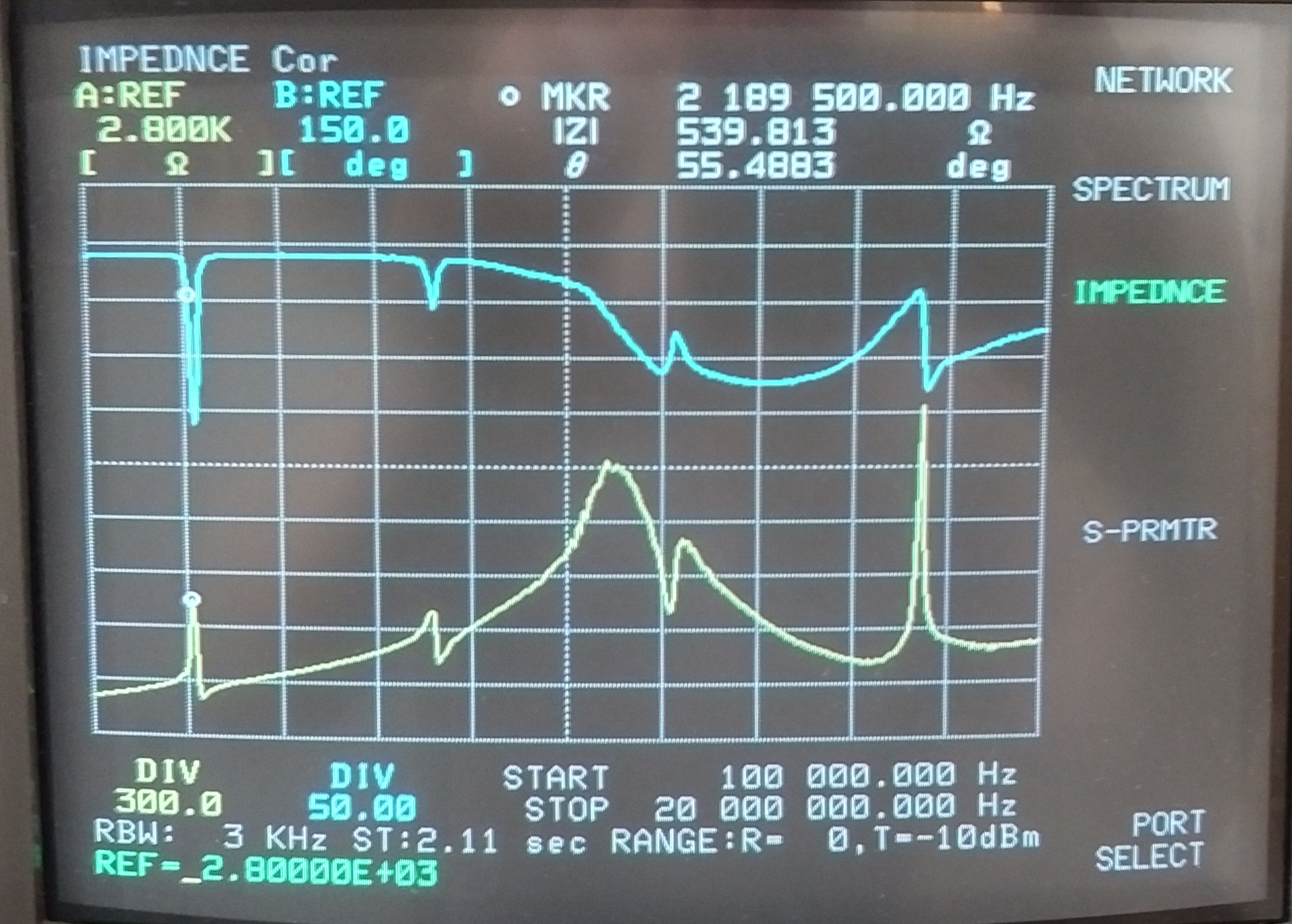
Fig 5.4. Shows the secondary added to form the flat coil 3S-1P where CP=0pF. As per Fig. 3.1 for the secondary and primary impedance-frequency responses become superimposed on one another. The primary resonance FP can be identified clearly at 11000kc/s along with the gradual phase chanhge, along with the secondary resonance FS at 2189.5kc/s with a variation of ~3% from the VNA-SDR measurement of 2254kc/s. Secondary harmonics can be identified in a similar way in a corresponding frequencies as per Fig. 3.1. The greater sensitivity and more finally tuned input circuits of the VNA-HP also show a strong additional resonance at FS4 at ~17.5Mc/s which is not identified in Fig. 3.1.
Fig 5.5. Shows primary capacitance CP= 830pF as per Fig. 4.1 where the lower resonant frequency of the flat coil FL has been adjusted to be at the designed frequency of 1850kc/s. The VNA-HP shows a close correlation at 1851.75kc/s ~1% variation, and corresponsing close correlation of FØ180 and FU.
Fig 5.6. Shows primary capacitance CP= 515pF as per Fig. 4.3. Here the FØ180 point is compared at 2390.75kc/s and 2418kc/s a variation of ~3%.
Fig 5.7. Shows primary capacitance CP= 650pF as per Fig. 4.5. Here the FU point is compared at 2819.5kc/s and 2875kc/s a variation of ~2%.
It has been shown that there is good correspondence of the key impedance features of flat coil 3S-1P when measured on both VNA-SDR and VNA-HP. The variation between measured parameters is acceptable for the intended purpose of the flat coil, and all the various measurements correlate well in drawing key conclusions regarding the impedance-frequency properties in part 2.
Summary of the VNA results and conclusions so far:
1. The fundamental resonant frequency impedance characteristics of the primary FP, have been shown to interact with that of the secondary FS to produce an upper and lower resonant frequency for the flat coil, FU and FL.
2. FU and FL can be adjusted in frequency by adjusting CP, which also leads to changes in |ZU| and |ZL|. Adjustment of CP allows the frequency band of operation to be selected, and occurs for FL within the target operation band, the 160m amateur band.
3. The balance of |ZU| and |ZL| leads to several important operating points for the experiments in displacement and transference of electric power. Most particularly when |ZU| = |ZL| and it is conjectured that the magnetic and electric fields of induction are in balance between the primary and secondary, which will lead to the best operating point for coherence between the induction fields and hence displacement events stimulated by non-linear events in the system.
4. The correspondence between measurements using different VNAs is good with variations in most key parameters being < 5%.
5. Equivalent circuit elements yield circuit values in reasonable correlation to those expected and those measured in part 1.
6. Small signal input impedance measurements Z11 have provided greater understanding and insight into the mechanisms governing the characteristics of the flat coil, how best to experiment using the flat coil, and how best to drive and match the coil to the various generators and loads.
Click here to continue to the flat coil impedance measurements part 3.
1. A & P Electronic Media, AMInnovations by Adrian Marsh, 2019, EMediaPress
2. Dollard, E. and Energetic Forum Members, Energetic Forum, 2008 onwards.
This part measures the coil impedance characteristics Z11 (magnitude and phase) for the flat coil in a range of different experimental scenarios. There are some preliminary results presented here in order to give an indication of the more complex frequency characteristics that exist within the experimental scenarios. The measurements and explanantion of the results presented here is still work in process and hence this post has not been fully finished at this time. As soon as time allows I will extend the range of measurements and experiments, and provide more detailed explanations and implications of the presented results. The impedance characteristics reported so far currently relate to the following experiments:
1. Two flat coils bottom-end connected via a load and being used for experiments in the displacement and transference of electric power.
2. Two flat coils bottom-end connected to the earth with ground rods and separated in distance by 250m being used for experiments in the telluric displacement and transference of electric power, (the generator flat coil in the lab, and the reception flat coil in the surrounding forest).
The details of these experiments will be reported in their own posts, although some pictures of the experimental arrangements are provided here for clarity, along with the preliminary impedance characteristics measured in those experiments.
Figures 1. show the experimental arrangements being used:
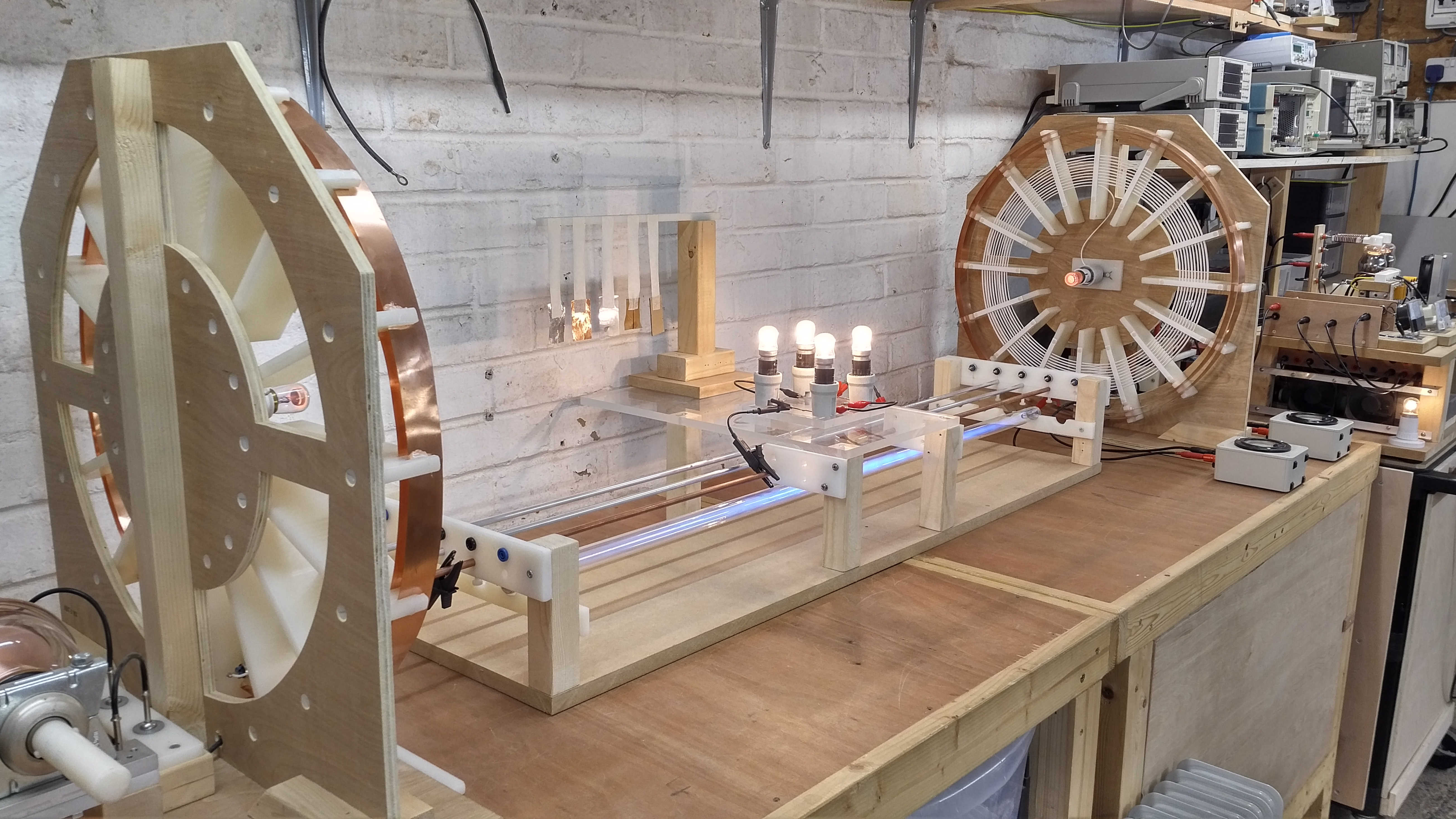
Fig. 1.1. Experiments in the displacement and transference of electric power.
Fig. 1.2. The generator flat coil 1S-3P.
Fig. 1.3. The vacuum tube generator driving the flat coil 1S-3P.
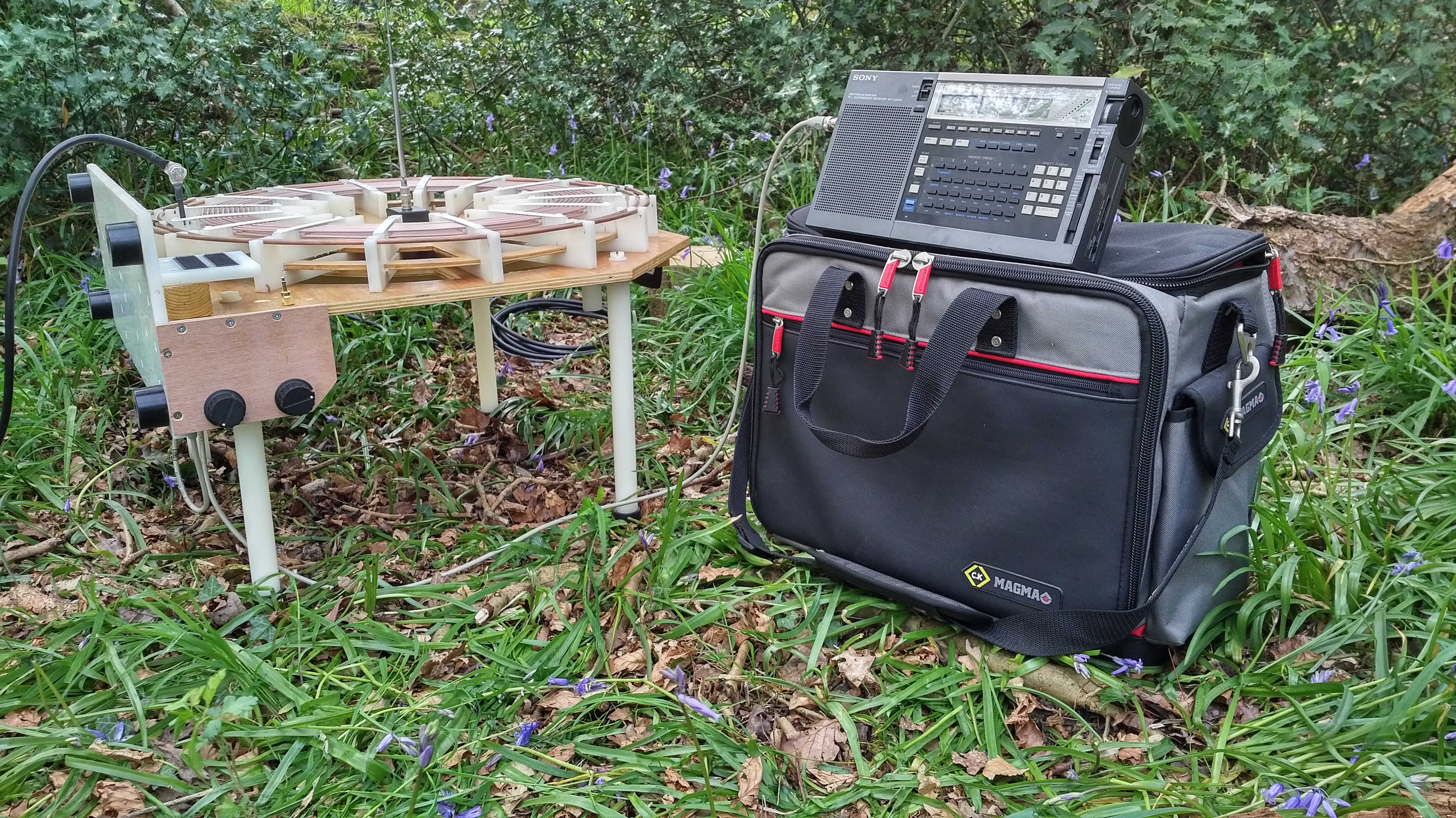
Fig. 1.4. Experiments in the telluric displacement and transference of electric power.
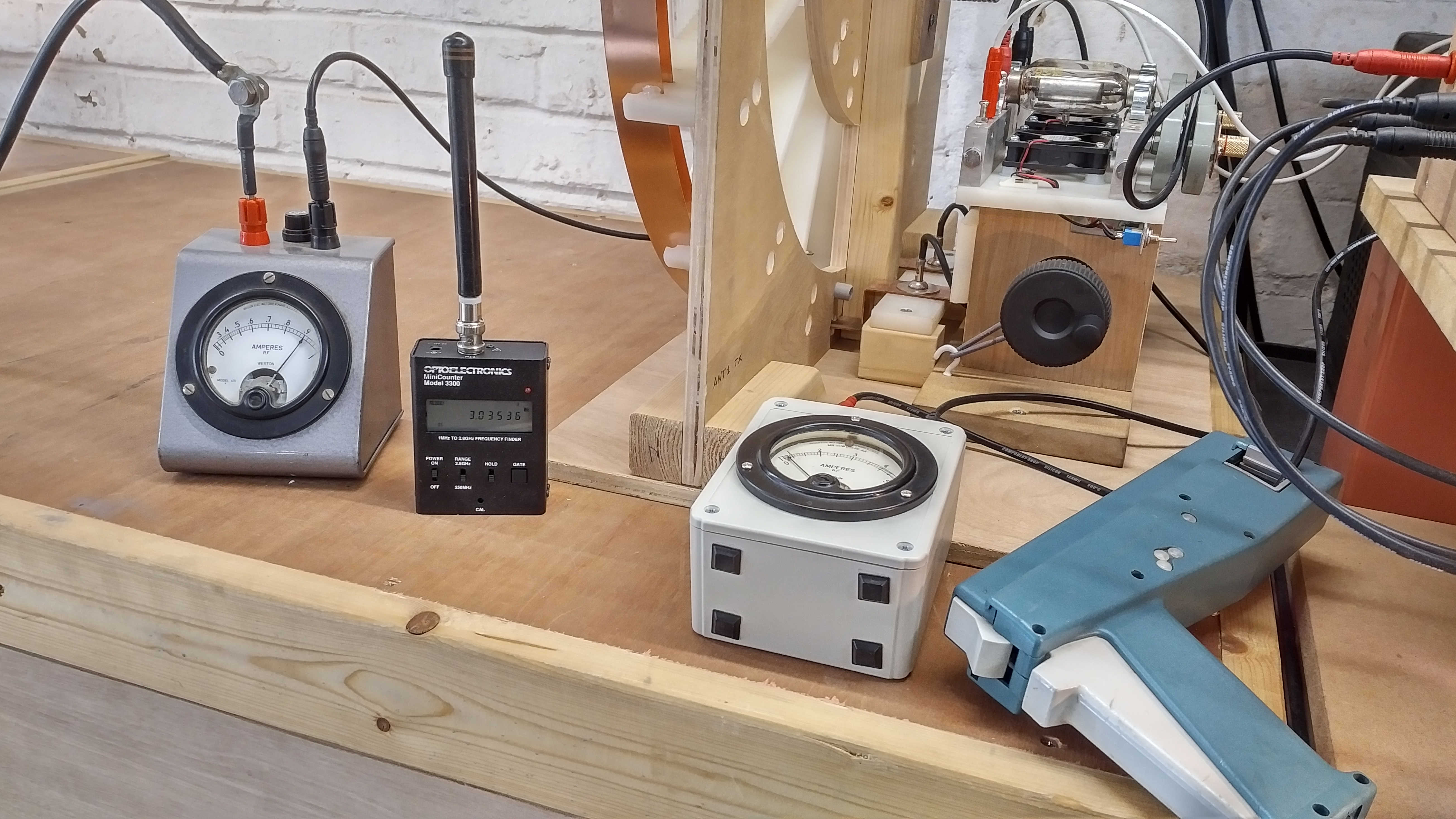
Fig. 1.5. Generator flat coil providing 0.9A rms at the upper flat coil frequency of 3.035Mc/s during telluric experiments.
Fig. 1.6. Flat coil 3S-2P being used in telluric reception tests and tuned to the upper flat coil generator frequency of 3.035Mc/s.
Figures 2. show the impedance characteristics measured for these experimental arrangements:
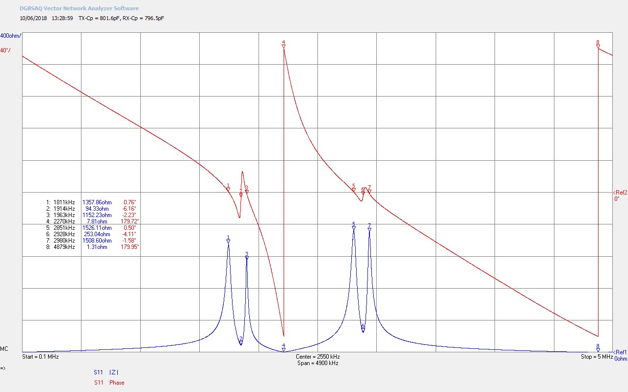
Fig. 2.1. Input impedance Z11 as seen by the generator for two flat coils bottom-end connected via a load and being used for experiments in the displacement and transference of electric power.
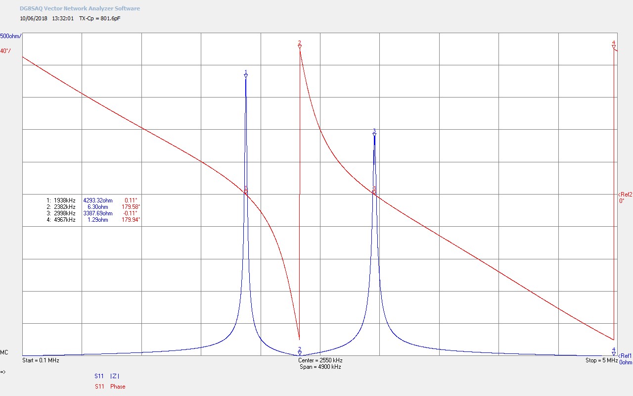
Fig. 2.2. Input impedance Z11 for the generator flat coil with bottom-end wire disconnected from the load.
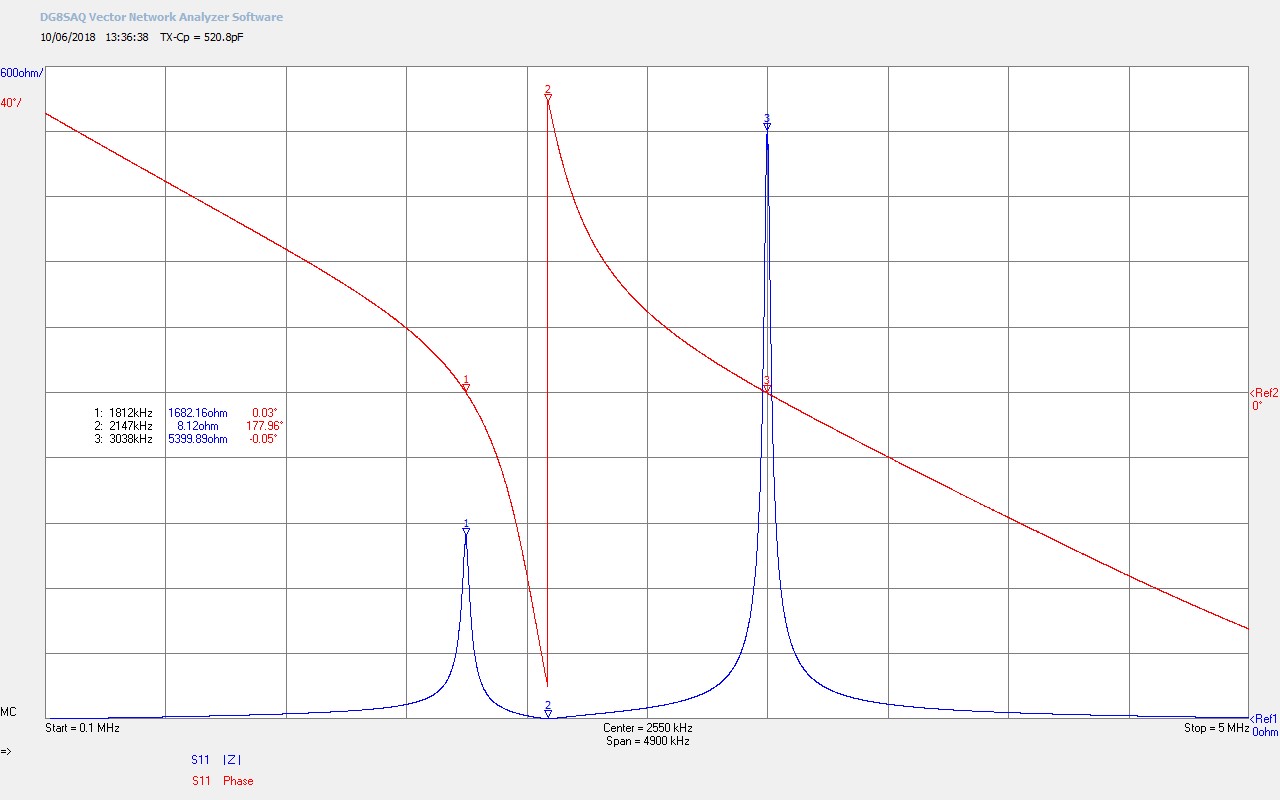
Fig. 2.3. Input impedance Z11 for the generator flat coil bottom-end connected to earth, and being used for experiments in the displacement and transference of electric power.
Note: this post is to be completed to include a more comprehensive set of impedance characteristics for the full range of experiments undertaken, along with their consideration, explanation, and implication to the purpose of the overall experiments.
Click here to continue to the flat coil single wire currents experiment.
1. A & P Electronic Media, AMInnovations by Adrian Marsh, 2019, EMediaPress
2. Dollard, E. and Energetic Forum Members, Energetic Forum, 2008 onwards.
Part 1 of single wire currents investigates the voltages and currents generated in the secondary coil, and connected load circuit, when the primary is driven from a suitable generator. In this part the generator used is a high voltage vacuum tube oscillator which derives the feedback for oscillation directly from the dominant flat coil resonant frequency.
The design, construction, and measurement of this generator, and its matching and tuning circuit, will be reported in subsequent posts. For clarity here the following different types of generator have been built and tested in a wide range of different experiments:
1. Vacuum tube generator driven either by an external high power oscillator, or directly as a self-tuned oscillator using feedback from the secondary coil. Can be driven in CW (carrier or continuous wave), burst, or modulated modes.
2. Spark gap generator, (static or rotary), driving directly a primary matching and tuning circuit, (tuning circuit as shown in Fig. 1.4 below).
3. Spark gaps driving a modern replica of an H.G. Fischer diathermy generator.
4. An original 1920’s H.G. Fischer diathermy generator.
Experiments in single wire currents investigate the interesting and unusual properties that result from high voltage and often high frequency waves emitted from a suitable source or generator and guided by a single wire to a load. The single wire nature means that power is passed from the generator to the load, and where the load is able to utilise this power to do work, through only a single wire. In a standard electric circuit a source of electric power such as a battery or an oscillator would be connected from both the +ve and -ve terminals for a current (dc or ac) to move around the circuit, and doing work in the circuit dependent on the characteristics and nature of the circuit. In this case if one of the terminals were removed, the circuit would be considered open-circuit, no current would flow, and no power could be utilised to do work within the circuit. In the single wire case the power conveyed through the electric and magnetic fields of induction easily do measurable work e.g. lighting an incandescent bulb, whilst the current in the circuit appears to be guided only by a single wire, that is, there is no obvious return wire for the current to pass back to the generator and create the required “circuit” for the classical conduction of electric current.
In part 1 of this experiment a vacuum tube generator is used to apply an rf sinusoidal (ac) current to the primary of the flat coil in CW mode. By extension of the magnetic field of induction to the secondary coil a magnified electric field of induction (emf) is induced across the secondary of the coil. When the secondary coil is further connected to a load via a wire at the bottom-end, or outer-end, an oscillating current (resulting from a reciprocal inter-action between the electric and magnetic fields of induction) is guided by the conductor of the wire to the load. In conjunction a pick-up coil is used behind the secondary to induce a small part of the magnified wave and feed this back to the vacuum tube oscillator. This positive feedback signal drives the oscillator at the dominant (tuned) frequency of the flat coil, in this case the lower resonant frequency FL at ~ 1850kc/s where CP ~ 900pF. In this way the circuit can be measured at a single frequency which can be tuned and adjusted using the primary capacitance CP.
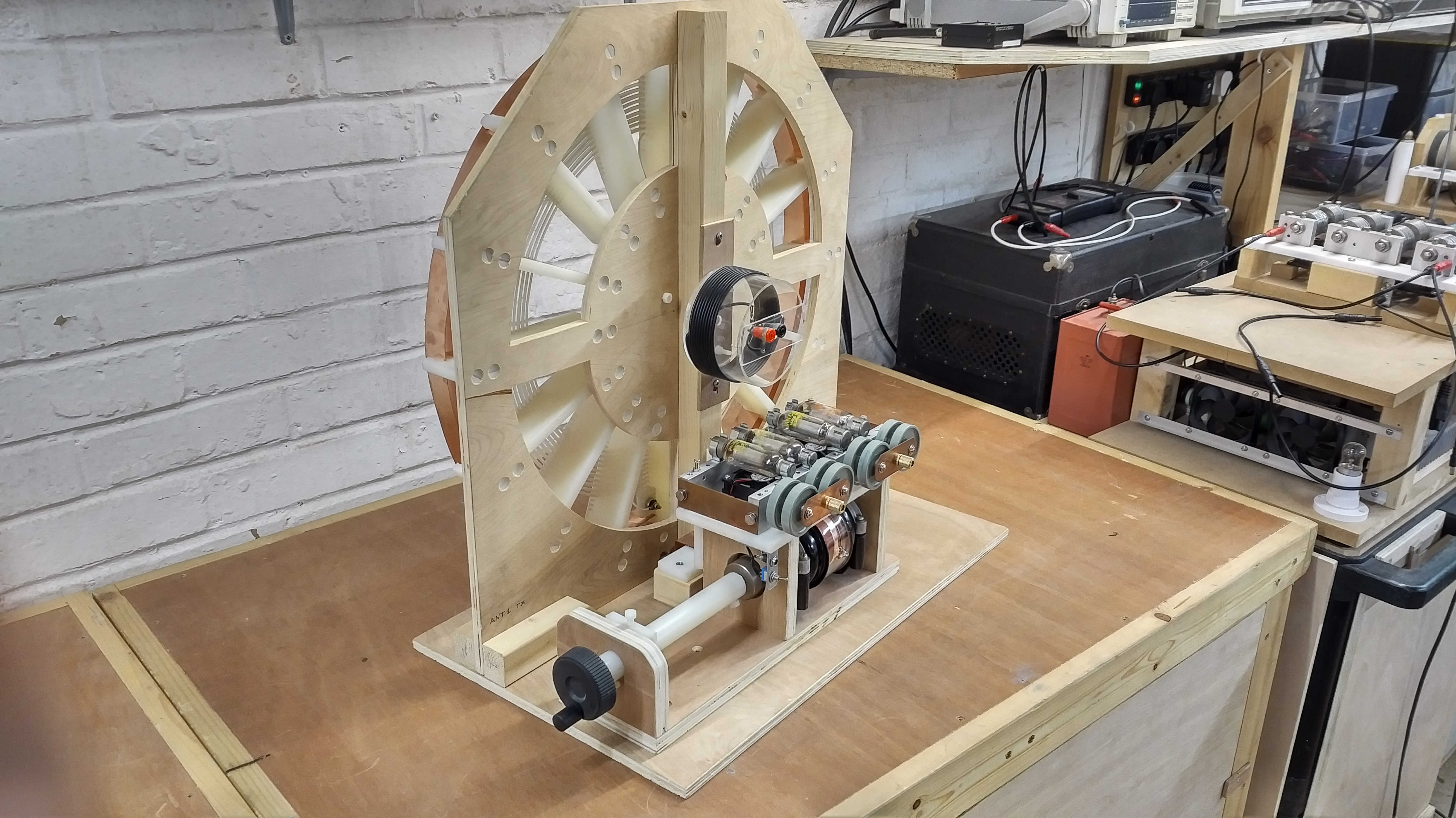
Figures 1. show the generator connected flat coil 1S-3P to be used in the single wire current experiments, and including the primary tuning circuit with primary capacitance CP, in this case a 4kV vacuum capacitor:
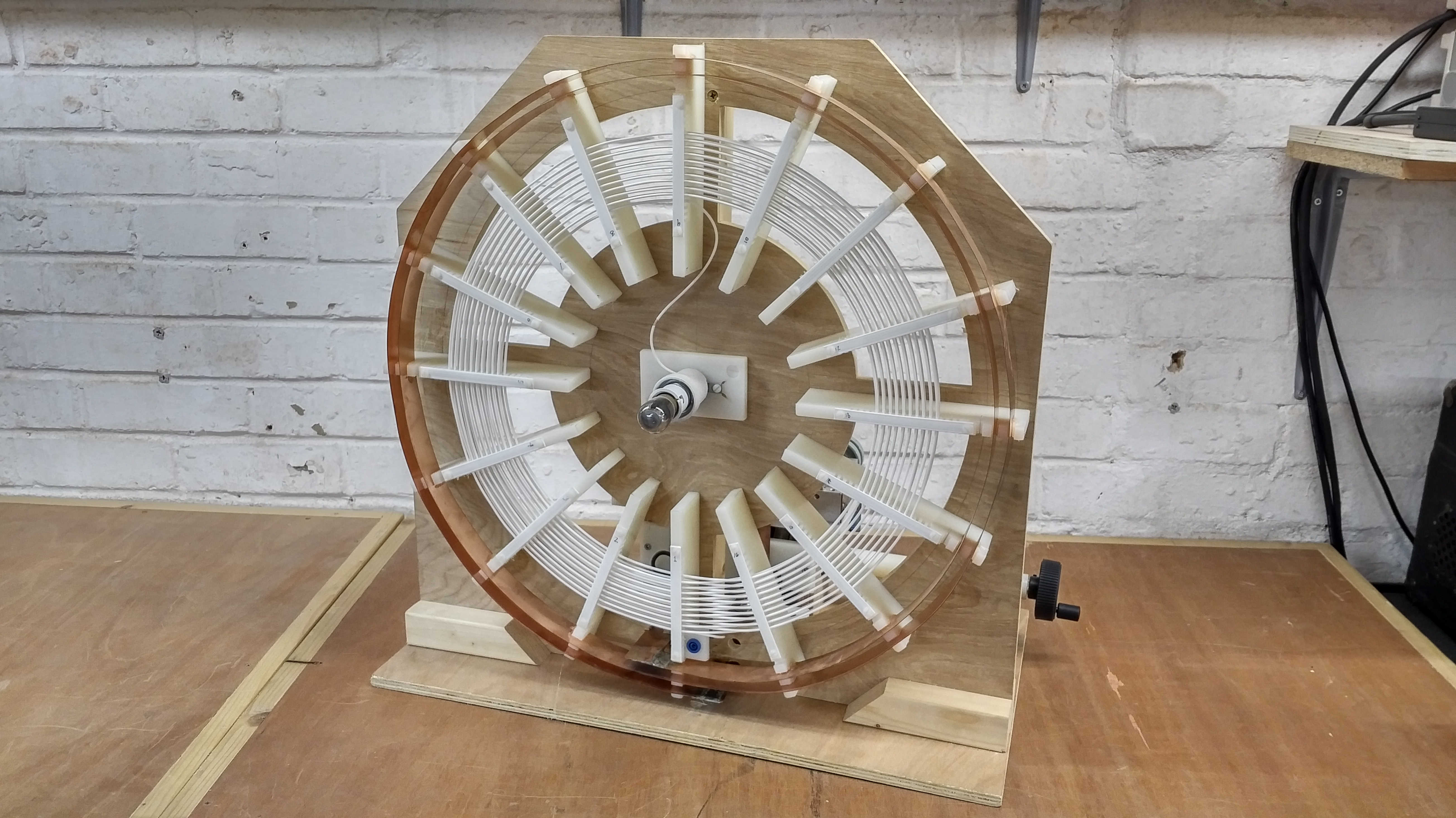
Fig. 1.1. Flat coil 1S-3P used as the generator coil for experiments in single wire currents.
Fig. 1.2. Flat coil 1S-3P constructed with PTFE coated multi-stranded wire, and copper strip primary.
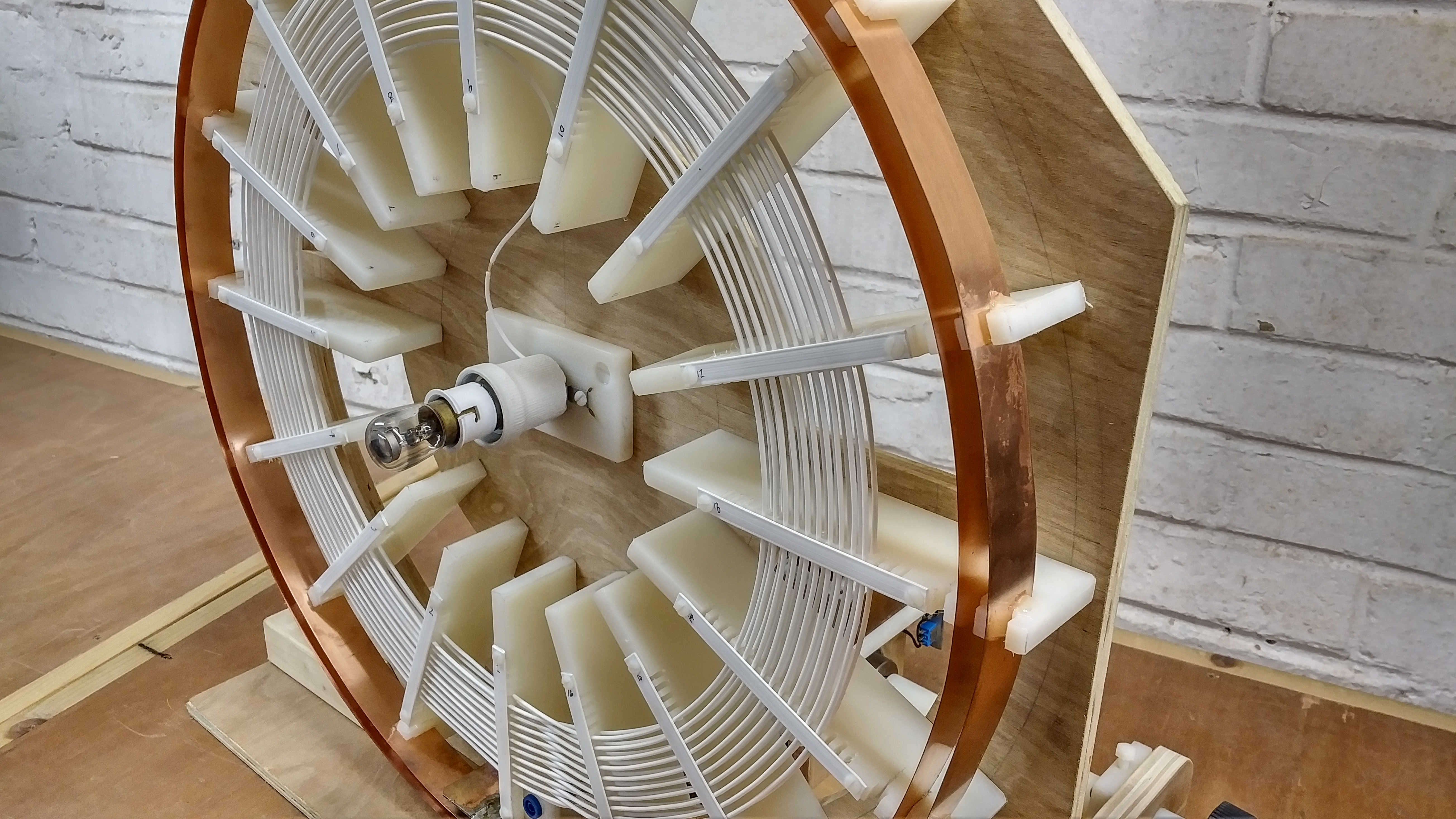
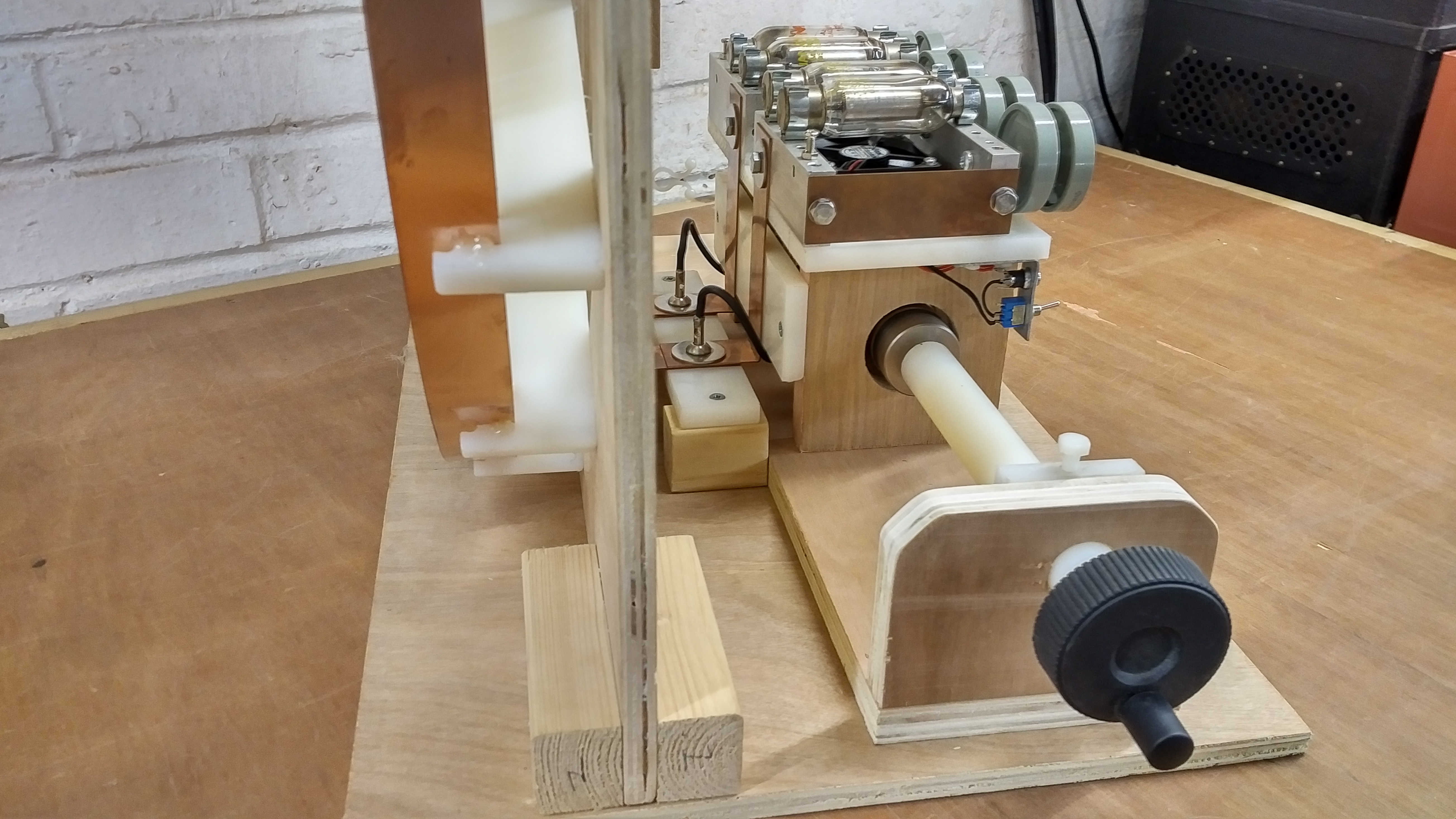
Fig. 1.3. Rear side of the flat coil showing generator feed and matching unit, and secondary pick-up coil to drive vacuum tube feedback.
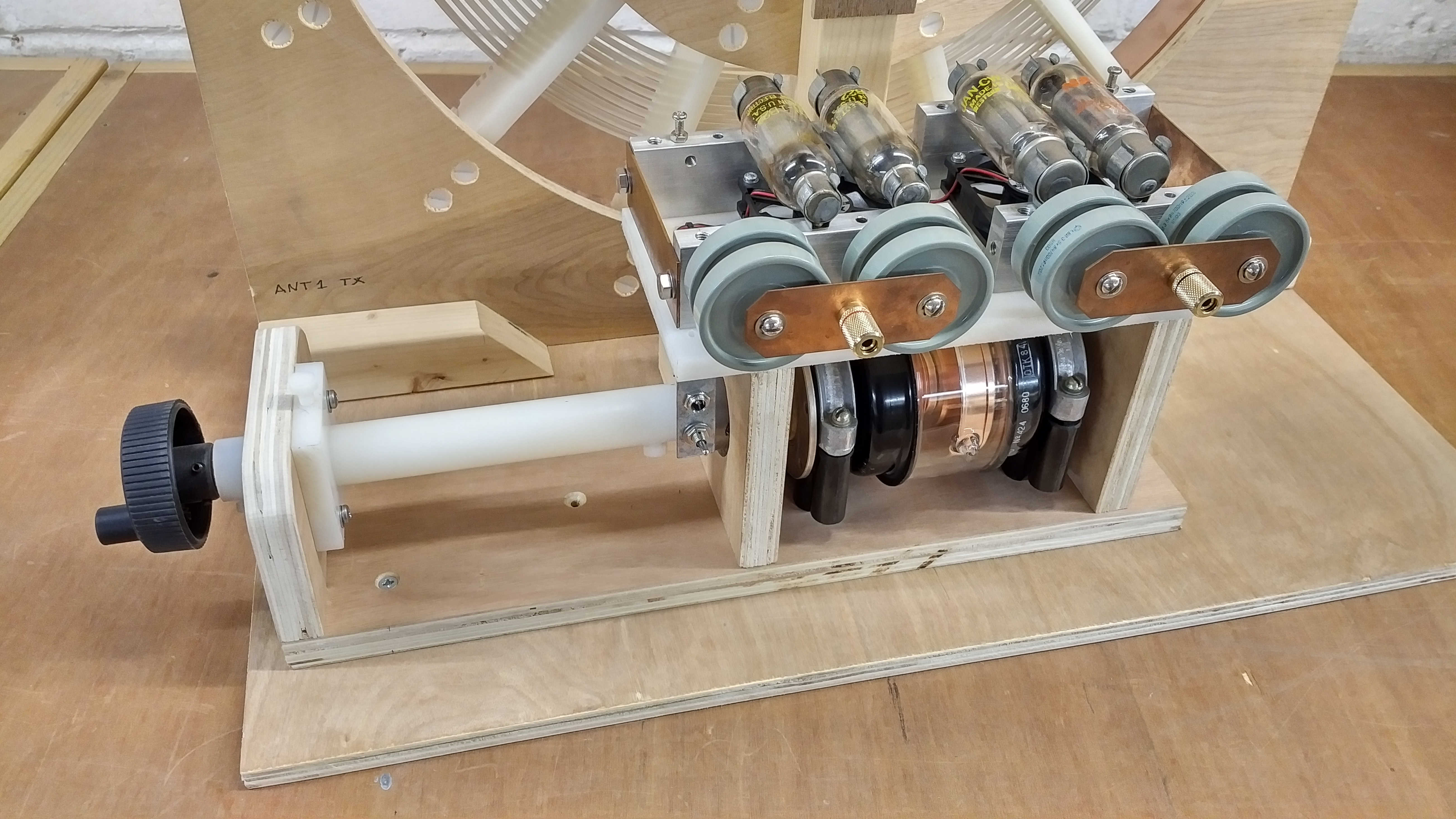
Fig. 1.4. Generator feed and matching unit consisting of the primary capacitor CP, and feed capacitors and 1B22 spark gap tubes for use with a spark gap generator.
Fig. 1.5. Generator feed unit is attached to the flat coil with copper strip and the primary capacitor is attached with silicone micro-stranded wire at the correct weight of copper connection point.
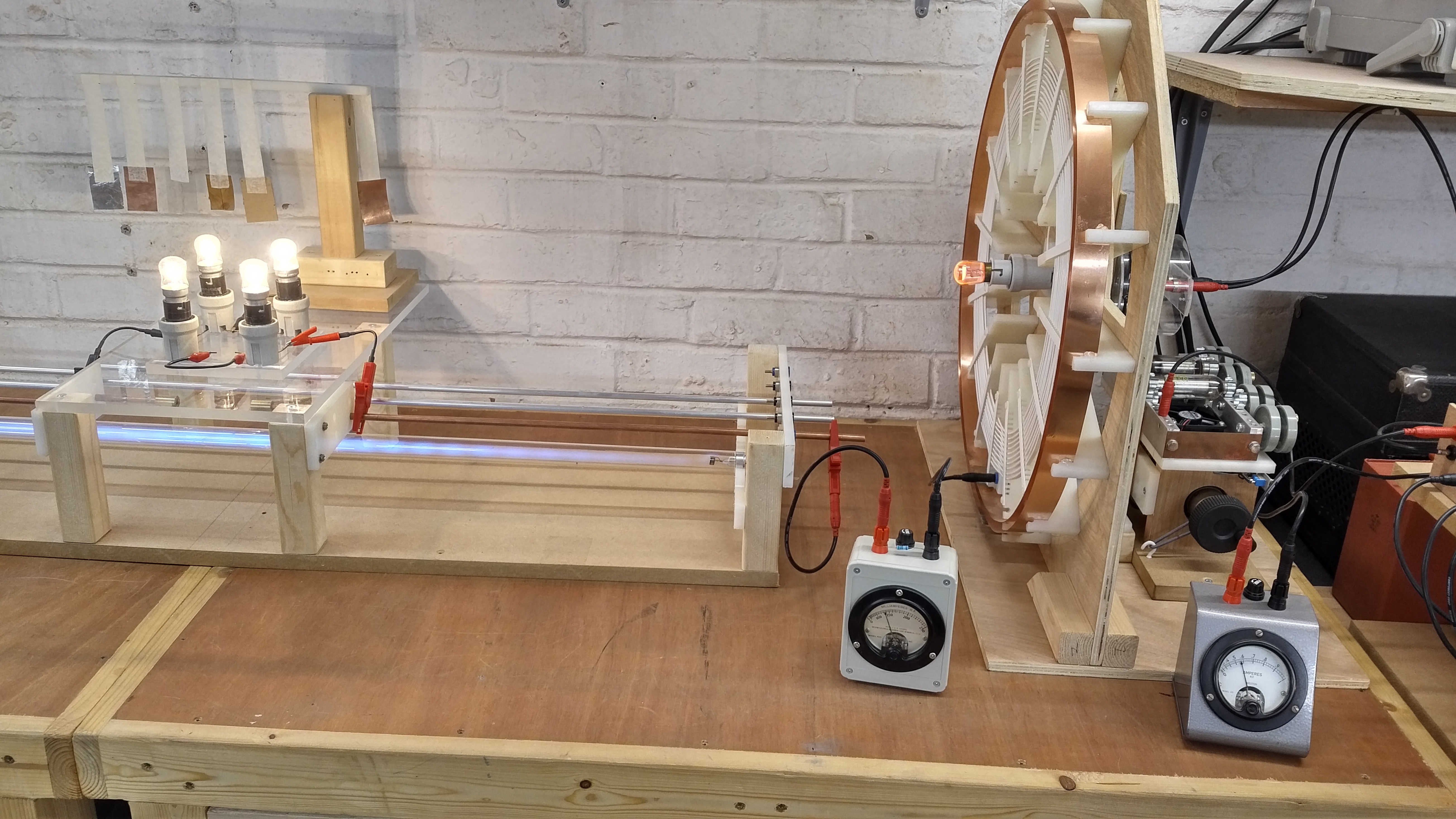
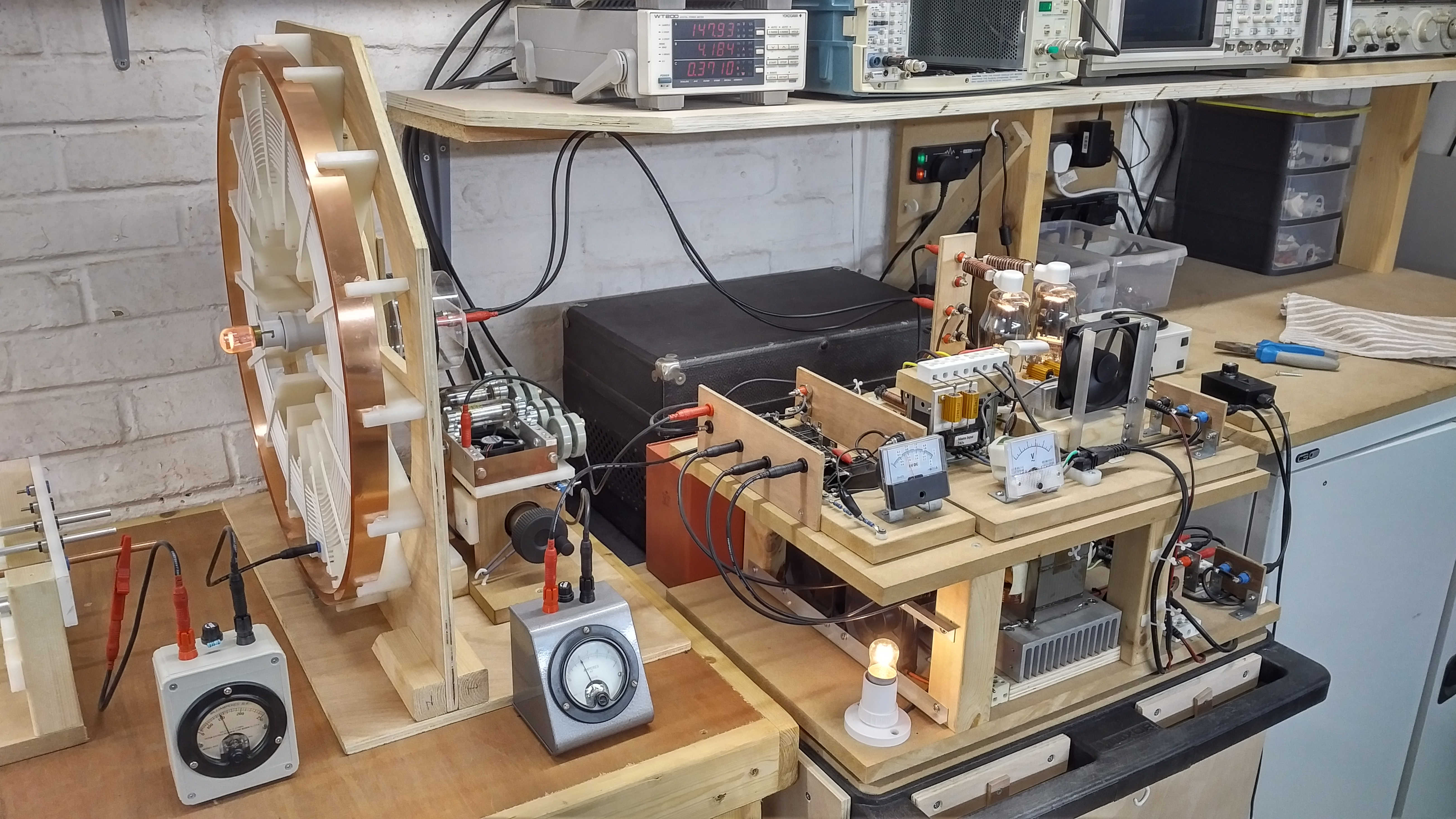
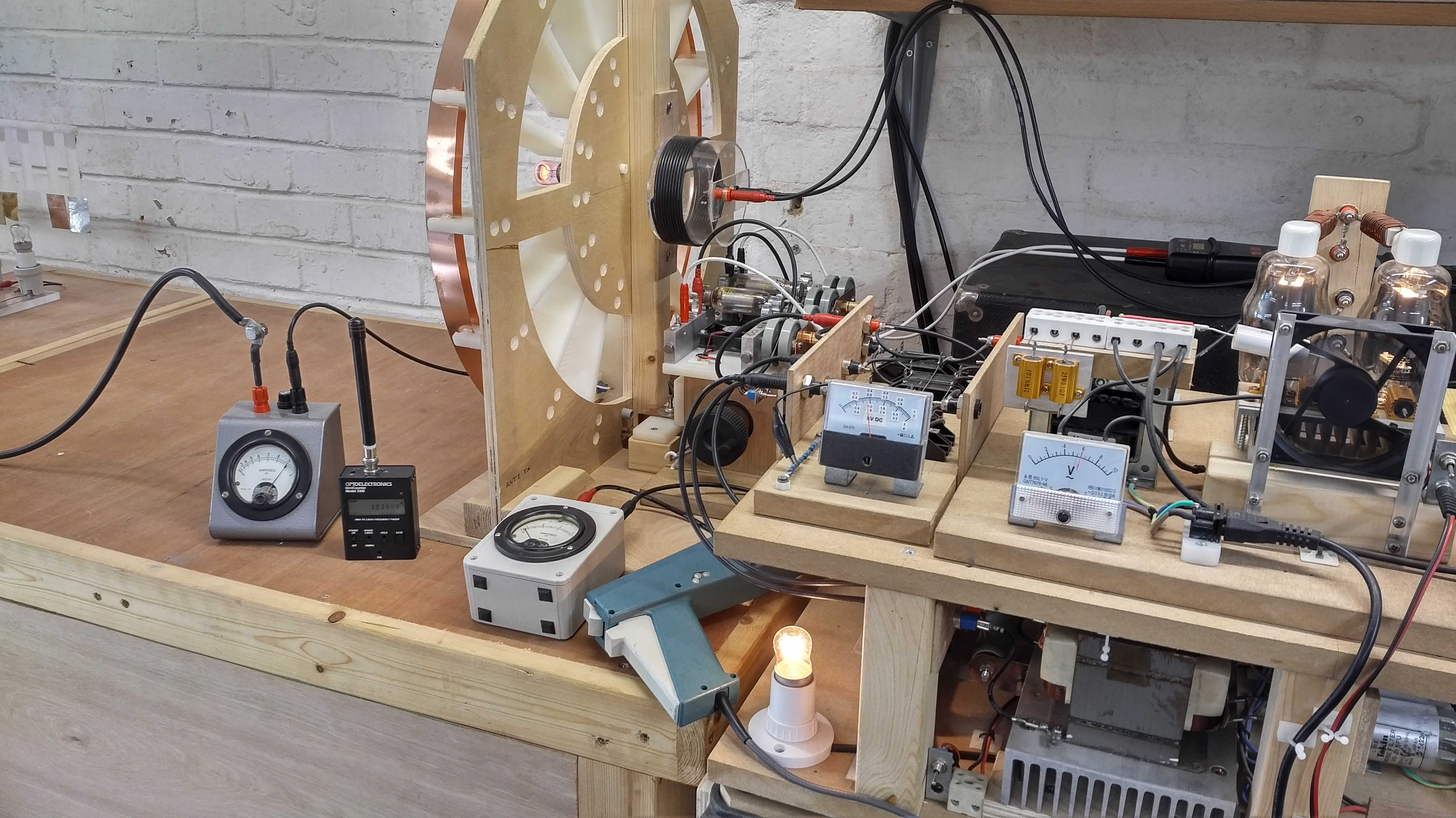
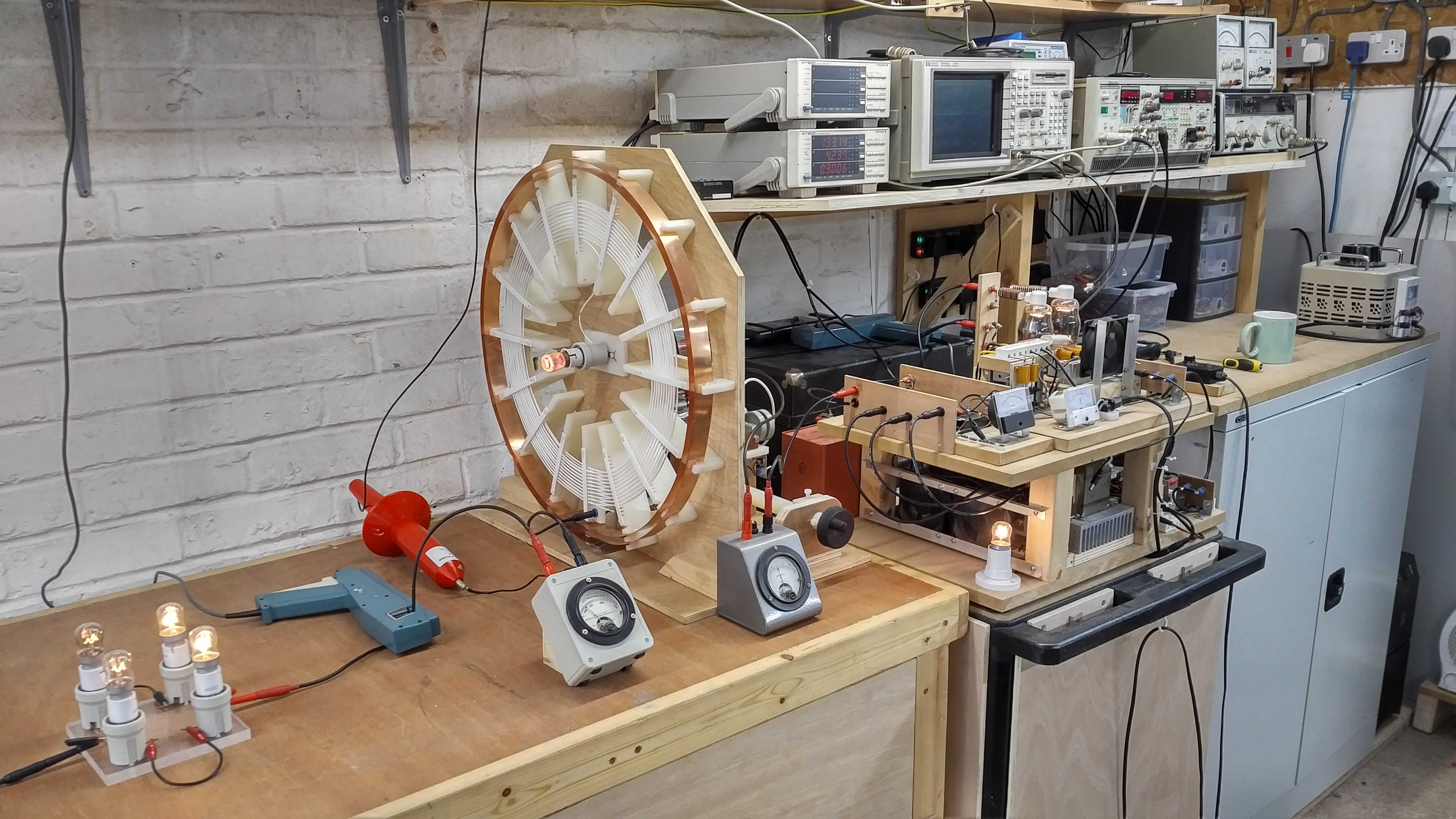
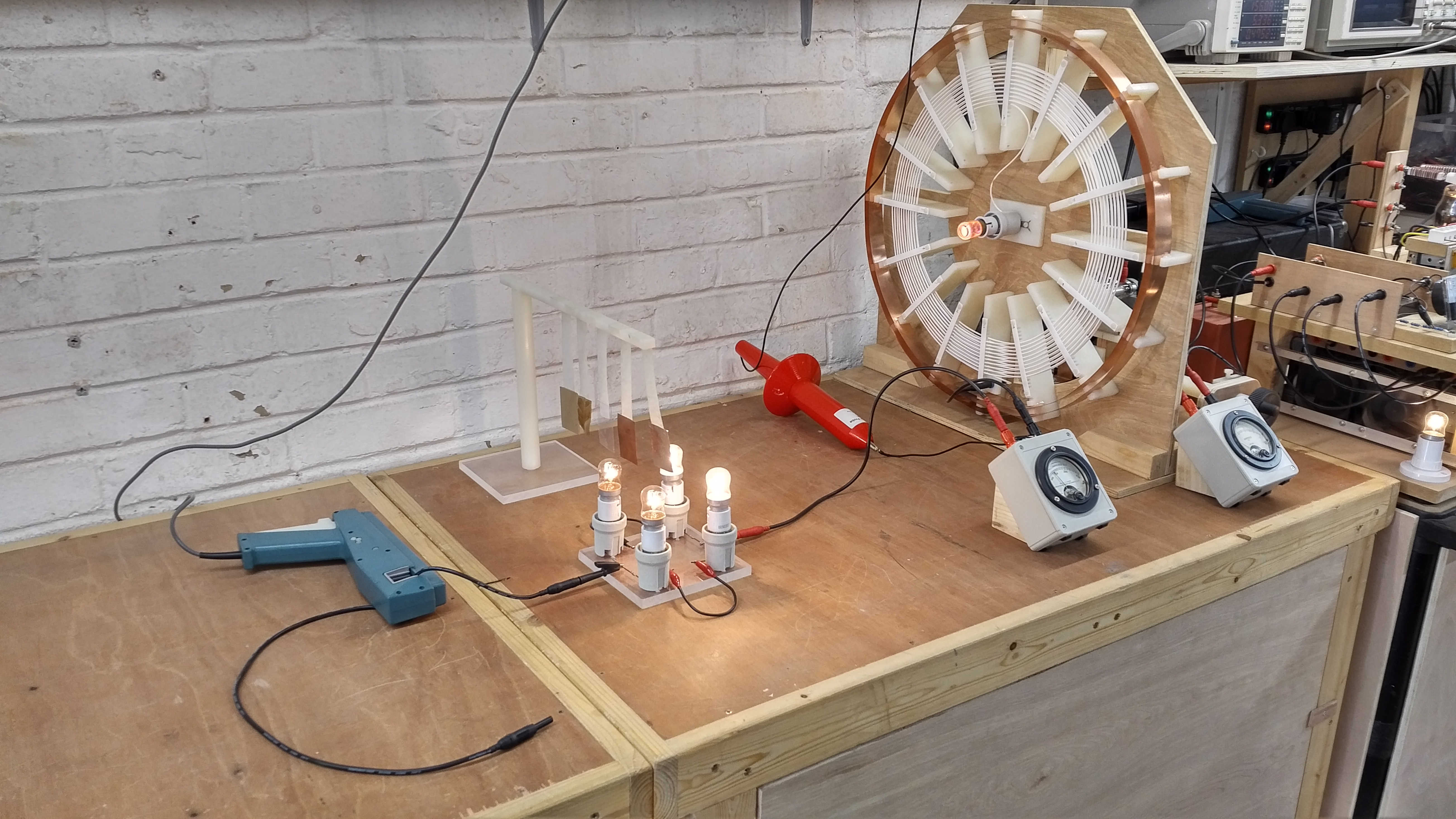
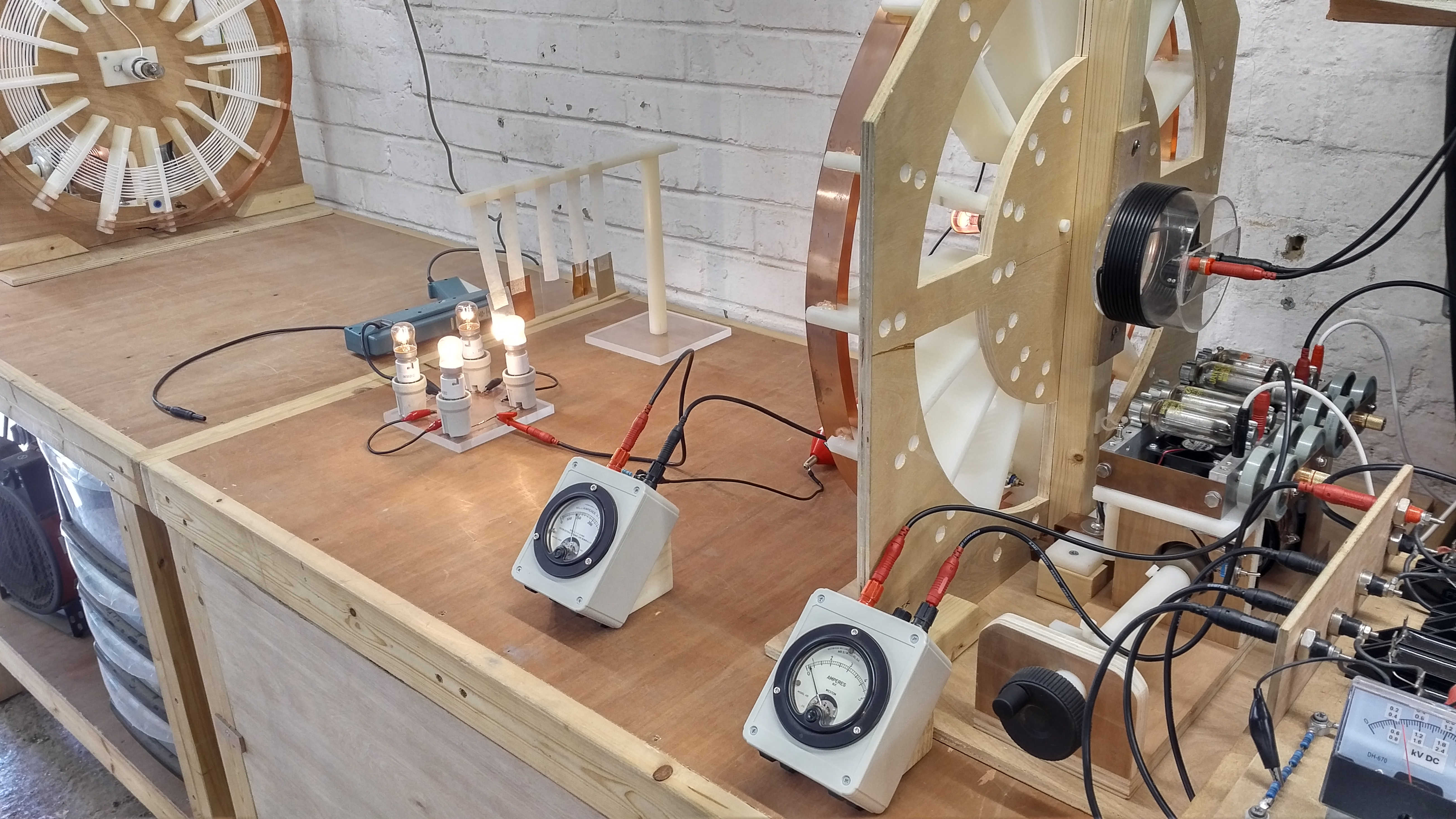
Figures 2. show the single wire current experimental apparatus, including measurement equipment and probes:
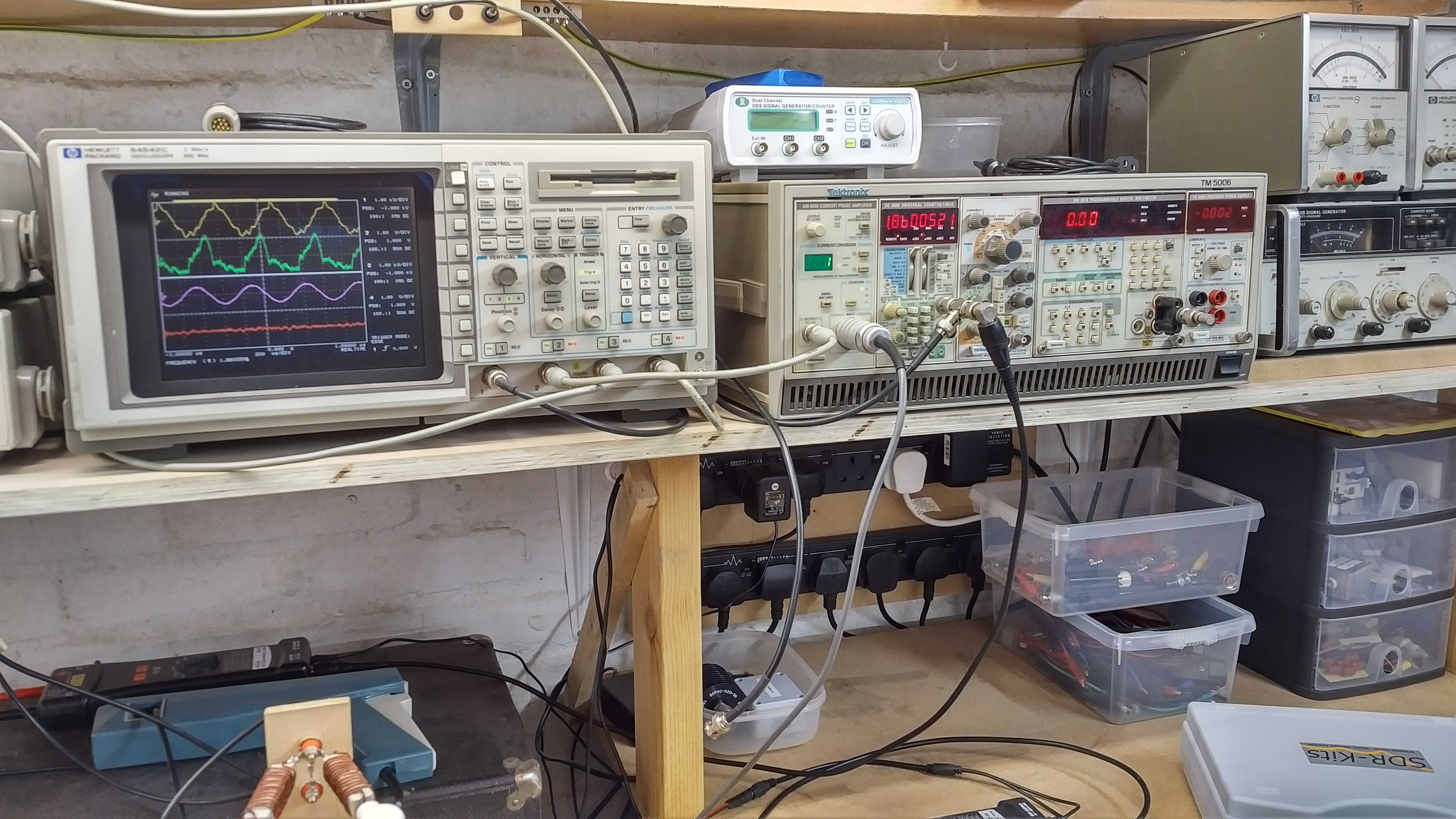
Fig. 2.1. Single wire currents experimental setup showing the vacuum tube generator, flat coil, load, probes, and test equipment.
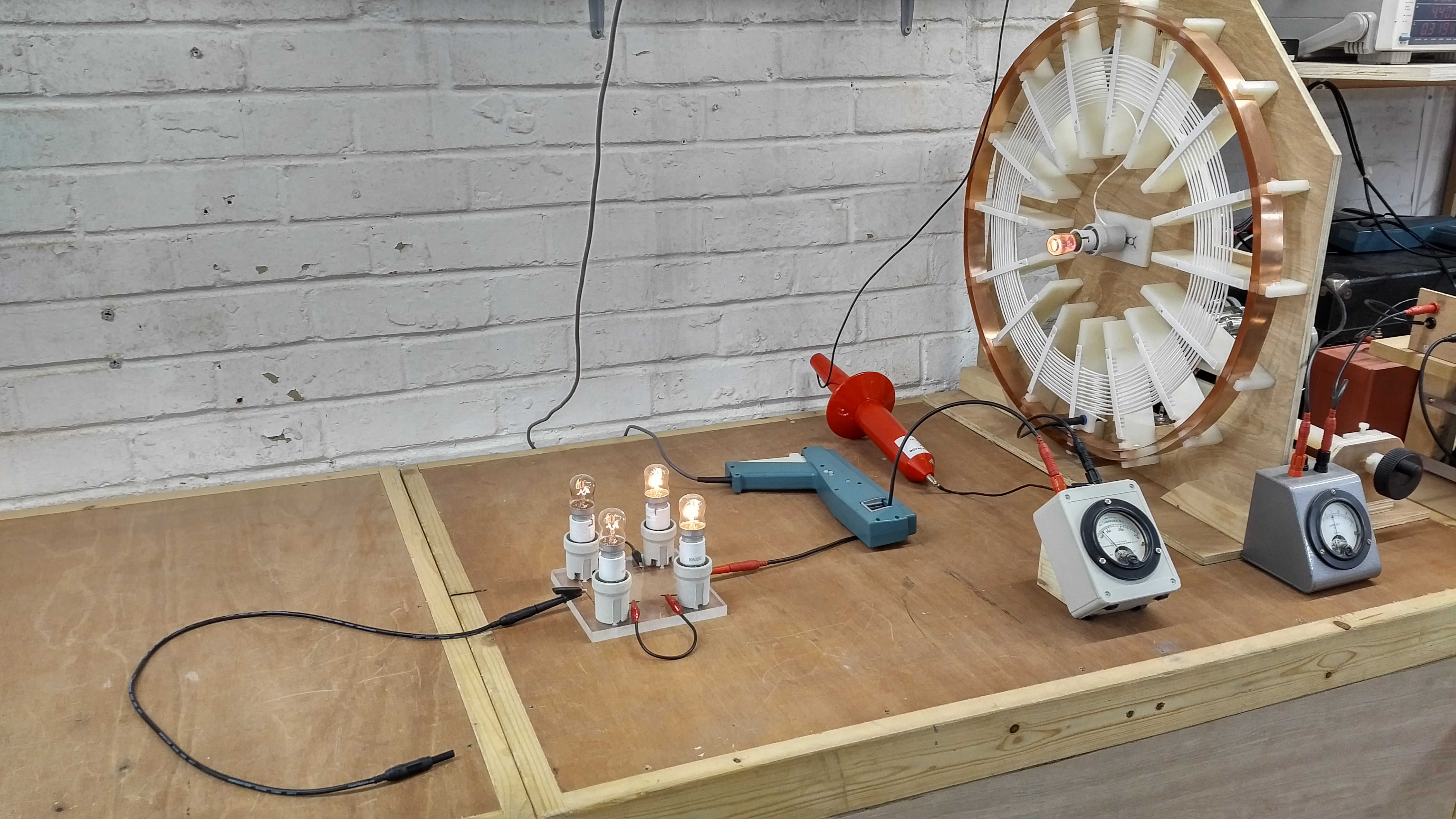
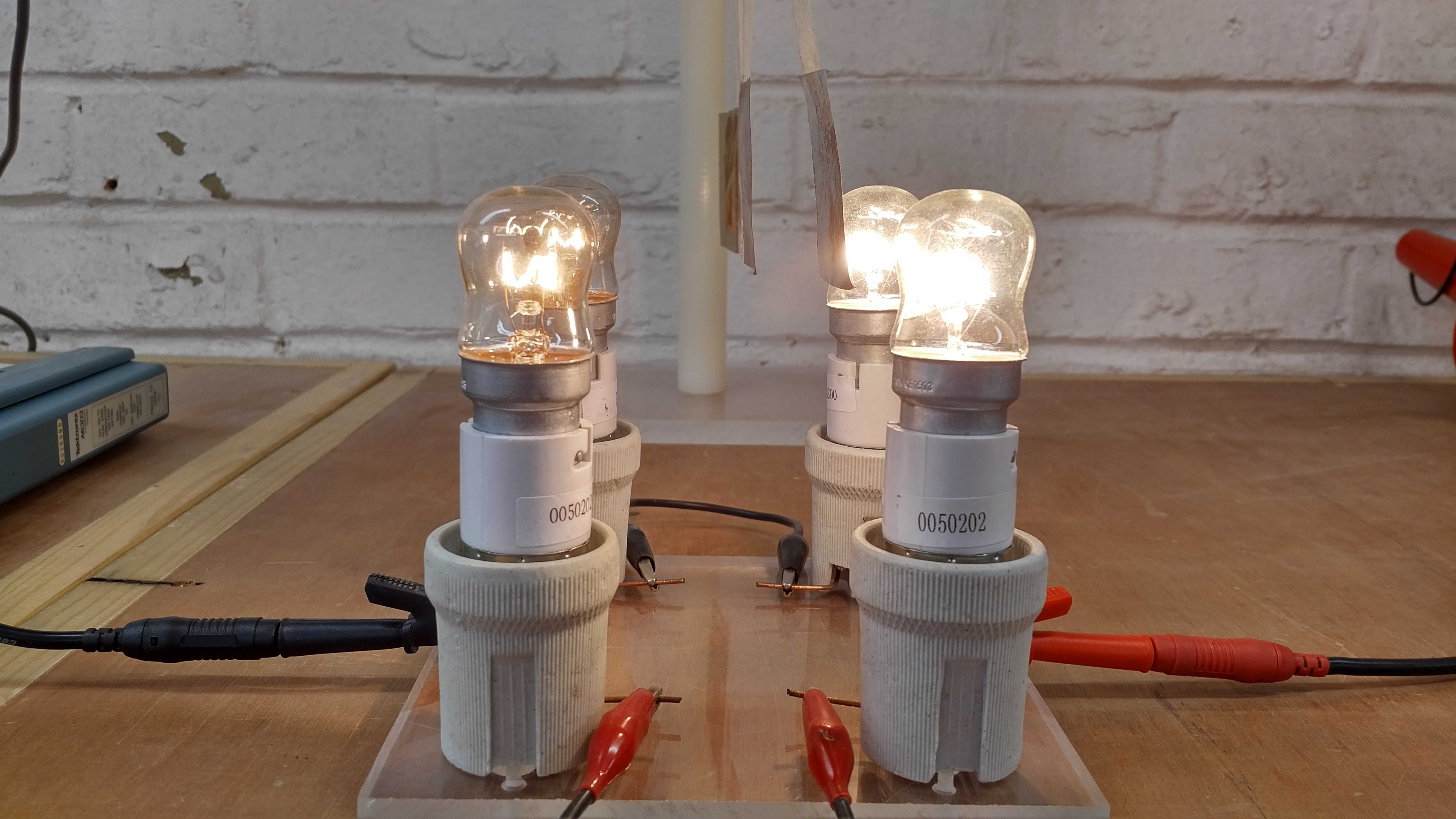
Fig. 2.2. The flat coil connected to the load bulbs via an RF current meter, and measuring secondary voltage and current. The output of the load is connected only to a single insulated wire.
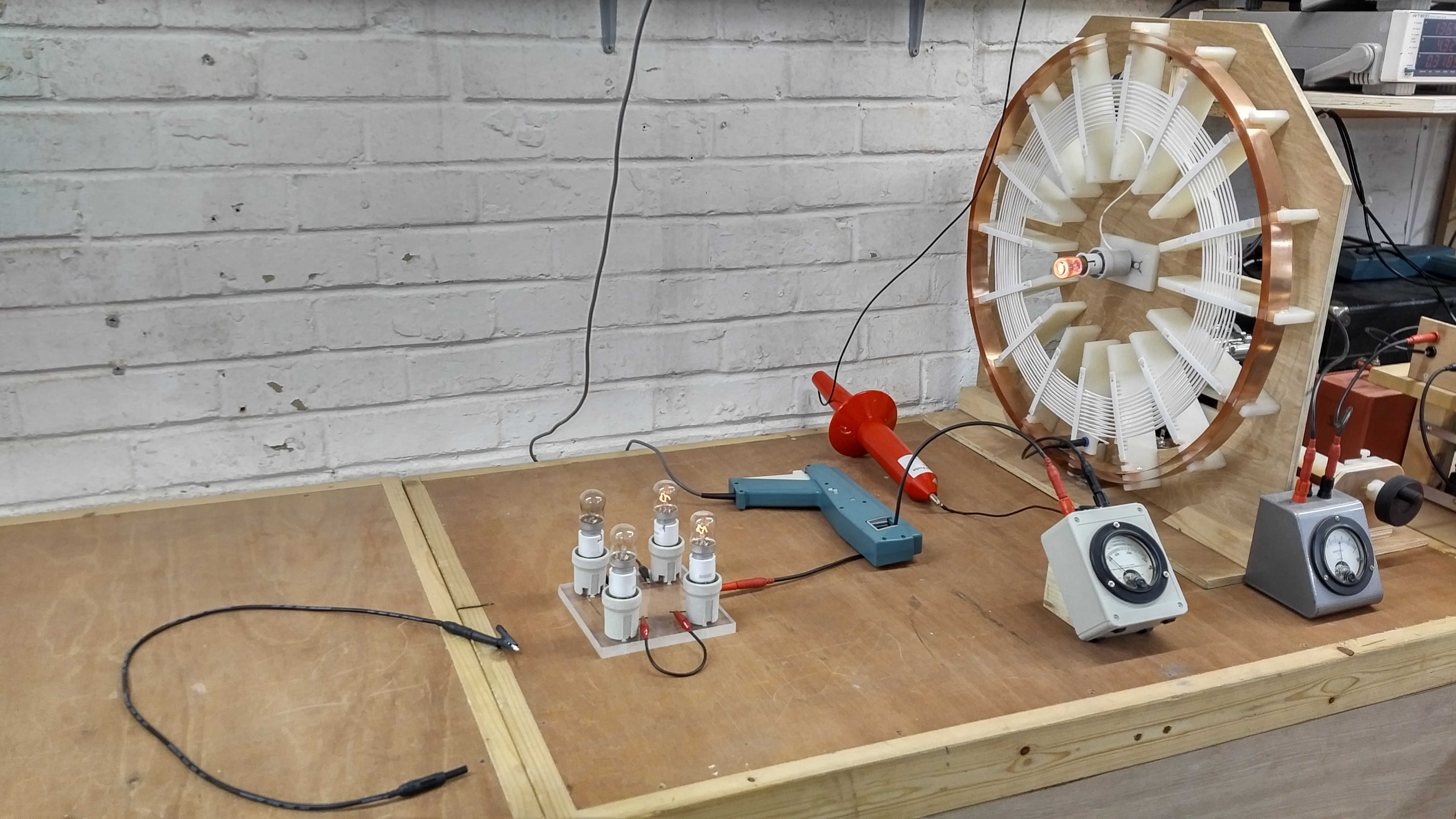
Fig. 2.3. Final load bulbs do not light when the output lead is disconnected.
Fig. 2.4. Aluminium leaf attracted towards the bulb load, and held in place whilst the generator is switched on.
Fig. 2.5. Aluminium leaf attracted to the bulb load, a source of light and rf emitter.
Fig. 2.6. Rear side of the generator coil showing matching unit connected to the generator, and rf current meters in the primary and secondary circuits.
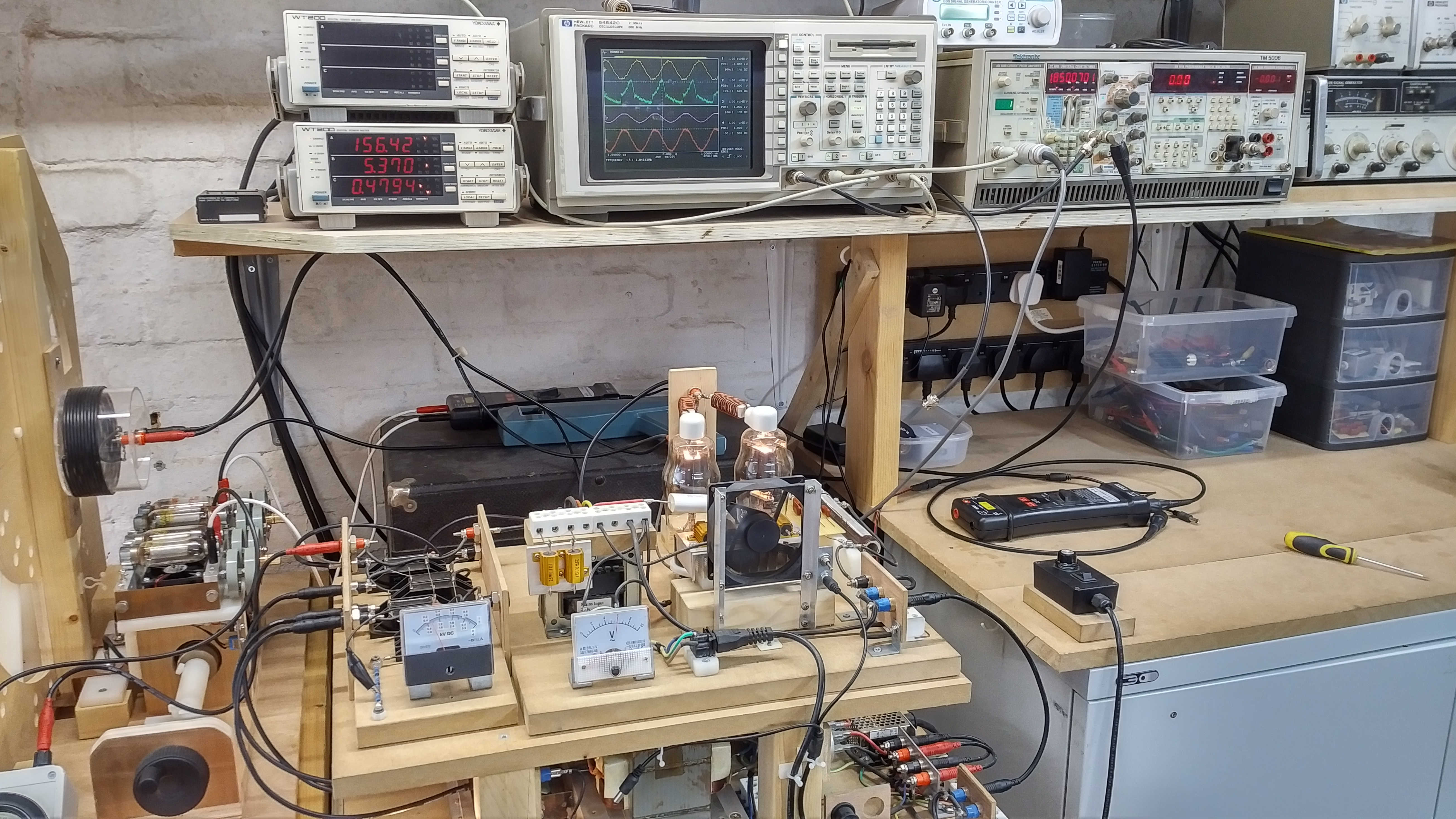
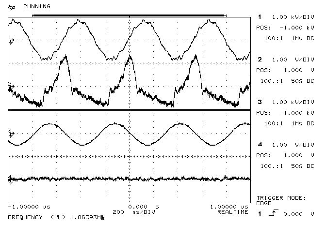
Fig. 2.7. Vacuum tube generator delivering 479W at 1850kc/s to the generator matching unit. Voltage and currents in the primary and secondary circuits are being measured using an oscilloscope.
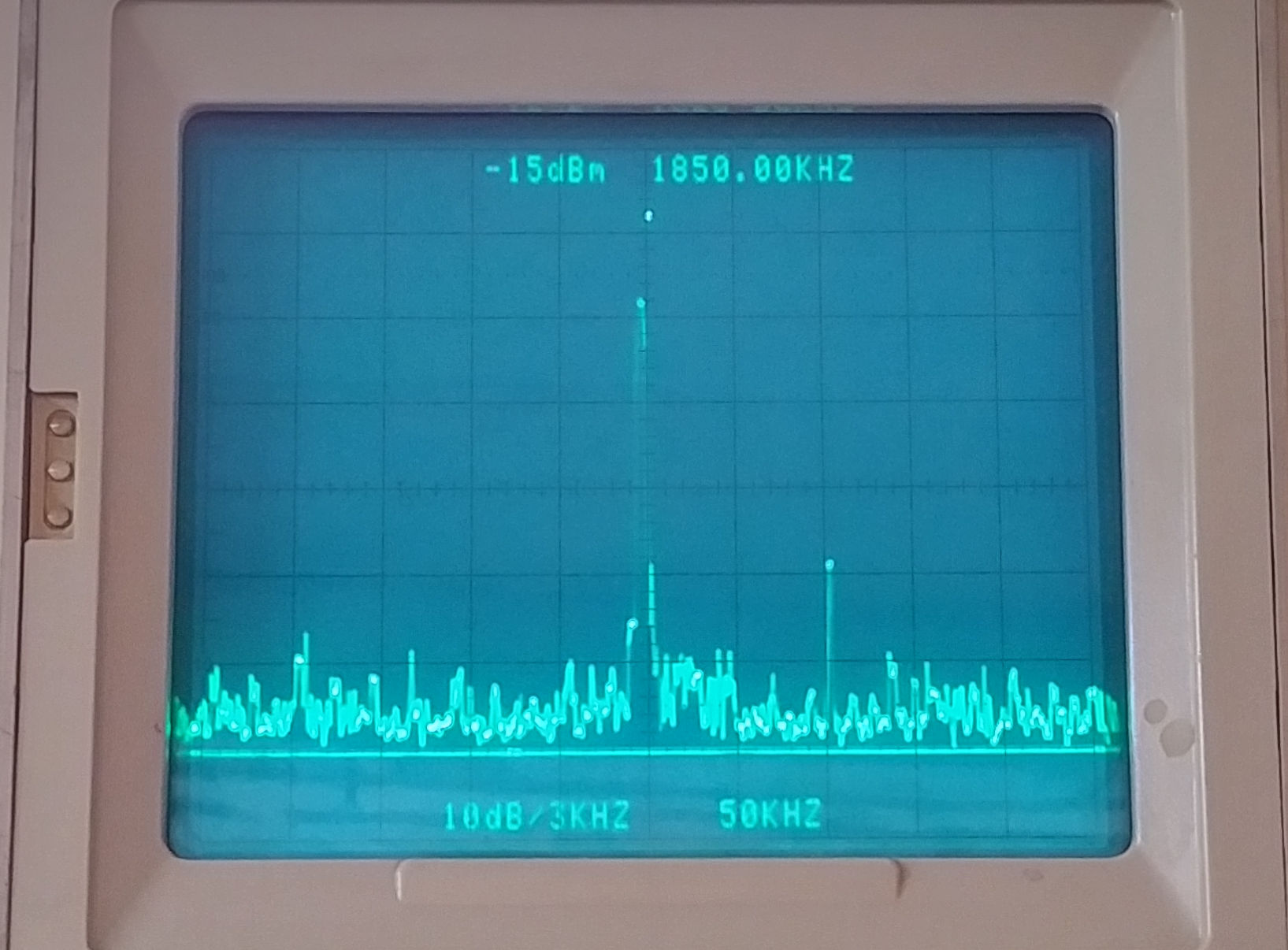
Fig. 2.8. Radiated power from the experiment is picked up by a small whip antenna connected directly to a spectrum analyser.
Fig. 2.9. With the load output wire disconnected the fundamental frequency has shifted to 1860kc/s, with no current measured in the output wire (red osciloscope trace).
To view the large images in a new window whilst reading the explanations click on the figure numbers below:
Fig 2.1. Shows the overall experimental apparatus, measurement probes, and equipment. The vacuum tube generator feeds the connections to the tuning unit with the primary capacitance. A high voltage differential probe Pintech DP-50 is connected across the primary capacitance to show the electric potential VP applied across its terminals. A current probe Tektronix A6303 is connected around the wire between the primary capacitor and the plates of the vacuum tubes to show the electric current IP moving through the primary circuit. Inserted between the high voltage tank capacitor and the input to the primary is a Weston model 425 rf ammeter (either 1A or 5A full scale deflection (fsd) dependent on generator output, and with internal thermocouple), to additionally monitor the primary rf currents IPRF.
In the secondary circuit the top-end of the flat coil is terminated with a 240V 5W (UK standard) neon bulb to act as an indicator of the magnitude of induced electric potential or tension, and to contain the top-end with a defined impedance. This containment assists in stabilising the resonant cavity formed by the secondary coil, and without significantly loading the coil and effecting the upper and lower resonant frequencies, or the Q-factor. The bottom-end of the secondary coil is connected by short wire to another Weston model 425 rf ammeter (250mA fsd) combined with a parallel 5Ω shunt to make 500mA fsd and to monitor the secondary rf currents ISRF.
The bottom-end of the coil is also connected to a high-voltage probe Pintech HVP40 40kV 1000:1 passive probe to monitor the secondary potential VS at the lower terminal. The output of the secondary ammeter is connected to the load, which in this case is 4 x 240V 25W (UK standard) pygmy bulbs with vertically laced filaments. The bulbs can be connected in a variety of arrangements, but were here used in a two parallel twin series connected arrangement so that all 4 bulbs will light as the load. The output of the load was connected to an 80cm flying lead. Secondary current IS was monitored in various places using a second Tektronix A6303 current probe.
The outputs of probes VP and IP from the primary, and VS and IS from the secondary, were passed to the inputs a four input oscilloscope HP54542C for measurement and comparison. In addition the signal VP was fed to a Tektronix DC5009 Universal Counter to confirm the oscillation frequency of the primary circuit. This frequency of oscillation was also monitored via a Tektronix 7L5 spectrum analyser fed by a small whip antenna at the input. Throughout the experiment the Tektronix current probes 2 x A6303 connected to AM503B current probe amplifiers were set on 1A AC /division. The total input power to generator PIN, (input to the high voltage transformers only), was monitored using a Yokogawa WT200 digital power meter.
Fig 2.2. Shows that at an input power of PIN = 319W @ 1851kc/s, IPRF ~ 700mA, ISRF ~ 240mA (2 x 120), and a 80cm fly lead connected to the output of the load bulbs, that all the bulbs are lit with the first two bulbs being lit brightly whilst the second two bulbs are only dimly lit. The measured waveforms will be considered in more detail in Figures 3.
Fig 2.3. Shows that under the same electrical conditions with the fly lead removed from the second load bulbs the intensity of the bulbs is greatly reduced. The first set of load bulbs are now dimly lit, whereas the second set of load bulbs are not visibly illuminated. ISRF has also reduced considerably to ~ 100mA (2 x 50mA), whilst IPRF increased slightly to ~ 770mA, at a PIN = 318W @ 1860kc/s. Here the frequency of oscillation has increased slightly due to the reduction in wire length with the fly lead removed, although vacuum tube generator has compensated automatically to shift resonance to the new resonant frequency via the secondary pick-up coil. The most important feature here is that in single wire current experiments loads will not power when no fly lead or terminating lead is connected to their output. In the case of a bulb it will not light when it is the last device connected to the single wire.
Fig 2.4. Shows the effect of introducing a conductive material close to the load in this case an aluminium leaf suspended by masking tape from an insulated support. Within a certain distance the aluminium leaf is attracted to the bulb outer glass surface and can remain held in this place until the generator is turned off. It appears a force is applied to the aluminium leaf that will move and/or retain the leaf in a distance offset from the vertical. This unusual result has been investigated in a variety of different ways and will be introduced here, to be further investigated and described in subsequent parts.
In the case of the CW vacuum tube generator (VTG-CW) the waveform induced in the secondary circuit is a steady and constant oscillation at a single frequency. This is a very linear and determinate condition and has been found to have the least intensity on the phenomena of attraction of conductive materials. At input powers typically 250W upwards in the experimental apparatus shown the aluminium leaf is very slightly attracted to the bulb glass. If placed only 1mm from the surface then the leaf will be pulled directly from vertical to a point on the glass bulb surface and held there. For distances x between the leaf and the bulb in the range 1mm < x < 15mm, and for the VTG in CW mode, the leaf can be held in place when initially placed on the bulb surface. Above ~15mm the aluminium leaf will not be retained on the bulb surface but will swing back to the vertical position.
The magnitude of the force applied to the aluminium leaf increases with the input power PIN to the generator and hence ISRF in the secondary wire. The overall effect is similar to observing a magnetic metal attracted to a magnet at close range, or the effect of electrostatic attraction in the case of opposite charged metal plates spaced slightly apart. In this case however it appears that the effect is based on the electric field of induction being dominant in the scenario rather than magnetic field of induction. When a permanent magnet is introduced into the experiment it has no influence on the attraction of the aluminium leaf either in being attracted towards the bulb, away from it, or being held on the bulb surface.
The intensity of the attraction and hence the magnitude of the applied force on the leaf has been found to increase significantly with burst, impulse, and modulated waveforms. With a burst or impulse waveform from the generator it is easily seen that at PIN > 400W the leaf can be instantly attracted to the bulb and move from the vertical over distances as much as 20mm, and then held there strongly on the surface of the glass. in this case even with the generator turned off the leaf can be retained for up to 60 seconds on the surface of the bulb before being released and swinging back to the horizontal.
Other types of leaf material have also been tested, and those found to readily be attracted and retained to the bulb glass have a conductive element to them, including metals like aluminium and copper, organic materials such as living tissue, plant matter (e.g. leaves), and paper, cardboard, and woods with a certain content of moisture in them. In the case of organic living tissue the presence of my hand in the vicinity of the light bulb, but not touching, greatly increases the effect even in CW mode. For man-made synthetic materials such as plastic and other insulating mediums there is normally no discernible attraction towards the bulb. At very high voltages and high input powers PIN > 1000W a plastic leaf was found to attracted to the bulb surface over a tiny distance < 0.5mm but could not be retained on the surface of the bulb even when placed directly on the surface.
With the aluminium leaf the voltage on the leaf was measured during the process of attraction and was found to rise to a high dc potential usually in the order of several hundred volts in the experiment thus described. This indicates a form of “charging” like the plate of a capacitor when exposed to a dc potential higher or lower than the surrounding environment. In this case the electric field of induction appears to have created a region of potential difference and tension between the material of the leaf, where the leaf has become “charged” to an opposite polarity than that present on the glass surface of the bulb. It is conjectured here that an electric wavefront (a positive dc level or impulse rather than a varying sinusoid) is emitted from the exposed wire of the bulb filament (itself a tiny extra coil and leading to an imbalance between the magnetic and electric fields of induction). These continuous wavefronts result in charge accumulation on the surface of the conductive material which establishes an electric field between the bulb filament and the conductive material. The electric field results in a force exerted on the aluminium leaf which is pulled towards the glass surface. As the conductors of the filament and the leaf are prevented to come into contact by the glass bulb the electric field is not collapsed by shorting the two together, and the leaf can be retained firmly on the glass surface as it remains “charged” by the presented wavefronts.
It is suggested that the attraction is not likely to be magnetic in nature, and as a result of eddy currents in the conductive material induced by the presence of a time varying magnetic field, as the phenomena cannot be influenced by other magnetic fields in very close vicinity, such as permanent magnets and electromagnets. It would be expected that the magnetic field generated by eddy currents in the leaf would be disturbed by the introduction of a strong permanent magnet, however no such disturbances have been observed or measured.
To eliminate effects due to convection and movement of air due to heating of the glass bulb a control experiment connected the same bulb type, a 240V 25W pygmy bulb, to a normal domestic ac outlet so that it would light to normal intensity and heating. The aluminium leaf was then placed in very close proximity to the bulb surface ~ 0.5mm with no discernible movement towards the bulb over any length of time the control experiment was conducted.
Fig 2.5. Shows in close-up detail the attraction of an aluminium leaf to the surface of the load bulb and being retained on the surface until the generator is turned off. In this case with the VTG in CW mode the attraction is not strong enough to pull the leaf from the vertical over a distance of 15mm to the bulb surface. The applied force is however strong enough to retain the leaf on the surface of the bulb at a distance of 15mm from the vertical, and once placed on the surface of the bulb.
Fig 2.6. Shows the experimental apparatus from the reverse side with the generator attached to the tuning unit, the rf ammeters in the primary and secondary, and the generator tank capacitor meter in the far bottom right showing a tank voltage of ~ 800V dc.
Fig 2.7. Shows the vacuum tube generator, primary measurement probes in the background, and the test equipment setup with PIN = 479W, the primary and secondary voltages and currents measured on the oscilloscope, and the measured oscillation frequency of the primary FP = 1.850Mc/s on the frequency counter.
Fig 2.8. Shows the spectral response of the emitted electric field in vicinity of the experimental setup and as measured by the Tektronix 7L5 spectrum analyser connected to a small whip antenna as shown in the bottom right of the picture. The spectral response shows a significant peak at ~1850kHz, and small possibly “artefact” peak at ~1950kHz.
Fig 2.9. Shows particularly the change in oscillation frequency measured in the primary circuit when the fly lead was removed from the output of the bulb load. The oscillation frequency of the experiment changes from ~1850kc/s to ~1860kc/s.
Figures 3. show the voltage and current waveforms for the primary and secondary and their phase relationship:
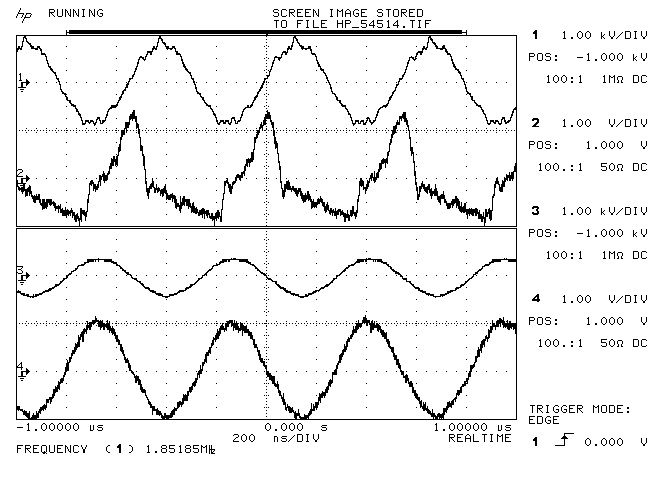
Fig. 3.1. Oscilloscope traces for primary (1,2) and secondary (3,4) voltages and currents. The output lead is connected to the load, all bulbs are lit.
Fig. 3.2. Oscilloscope traces for primary (1,2) and secondary (3,4) voltages and currents. The output lead is disconnected from the load, final bulbs are not lit, and secondary current is monitored in the disconnected load wire.
Fig. 3.3. Spectrum analyser signal picked-up using a small whip antenna positioned 3m from the experiment, and showing the resonant frequency at ~1850kc/s.
Fig 3.1. Shows the primary and secondary voltage and current measurements VP (trace 1) and IP (trace 2), and VS (trace 3) and IS (trace 4) respectively. VP is a sinusoidal oscillating voltage VPK-PK ~ 2kV. IP is more in the form of a pulsed current where the trace is calibrated 1V per amp and showing IPK-PK of ~ 2A. The phase of the current IP is leading VP by ~90° indicating that the generator appears to be driving a reactive load that is predominantly capacitive in a class-C amplifier arrangement. This is to be expected as the 180° phase change of the primary has been shown to exist at a much higher frequency than the impedance maximum for the primary would indicate. Operated in this way the primary and secondary are not at resonance simultaneously, the primary circuit is oscillating with a driven ac, whilst the secondary is acting as a free resonator at its tuned resonant frequency which determines the driven frequency in the primary.
As the voltage VP rises across the primary the current IP is maximum and falls rapidly as the primary capacitor CP is charged by the tank capacitor, on which that energy is released through the inductance of the primary coil reversing the current flow and discharging CP. This yields current pulses of sufficient magnitude for the magnetic field of induction to dominate and extend to the secondary coil. The secondary coil is not tightly coupled to the primary and so can reasonably resonate freely as the generator oscillates at a frequency determined by feedback from the secondary to the generator pick-up coil.
Using the VTG in cw mode it is important to note that the secondary is constantly being excited by the primary in a linear continuous fashion. There is no charge and discharge phase in the secondary as would occur in a burst or impulse driven primary. In this case the VTG is driving the flat coil in a very linear condition where the system operates at one set frequency, and the dominant majority of energy is conveyed at the fundamental resonant frequency, with very little contribution from harmonics. In this case we would expect phenomena that arise from the imbalance between the electric and magnetic fields of induction to be minimal, which is so far confirmed by measurement of single wire phenomena including deflection of conductive materials, and dc charging of capacitive loads.
The freely resonating secondary shows VP and IP which are in phase in traces 3 and 4, which is to be expected for a freely resonating coil driven with a very linear continuous wave. VS at the bottom-end or outer-end of the secondary coil is ~1kVPK-PK, and the current IP measured by the current probe prior to the load (as shown in Fig. 2.2) is ~ 2APK-PK (1V per amp calibrated on the current probe amplifier).
Fig 3.2. Shows the change in waveforms when the fly lead is removed from the end of the load, and the secondary current probe is connected through the fly lead. The frequency of oscillation has increased due to the reduced wire length in the experiment to ~1860kc/s (as measured by the frequency counter and spectrum analyser, rather than the marker frequency of the oscilloscope). The primary waveforms VP and IP remain largely the same in amplitude, phase, and form. The secondary voltage VS has increased as the effective load is reduced in the secondary, and IS has gone to zero as the fly lead, from which the current is being measured, has been disconnected from the output of the load. In this case the final load bulbs were not lighted, and the first load bulbs were lit only dimly with a significant reduction in ISRF.
Fig 3.3. Confirms the electric field detected in the vicinity of the experiment throughout the measurement period, where the pick-up whip antenna is located ~ 3m from the load bulbs.
To view the large images in a new window whilst reading the explanations click on the figure numbers below:
Figures 4. show the Z11 input impedance characteristics of the experimental apparatus:
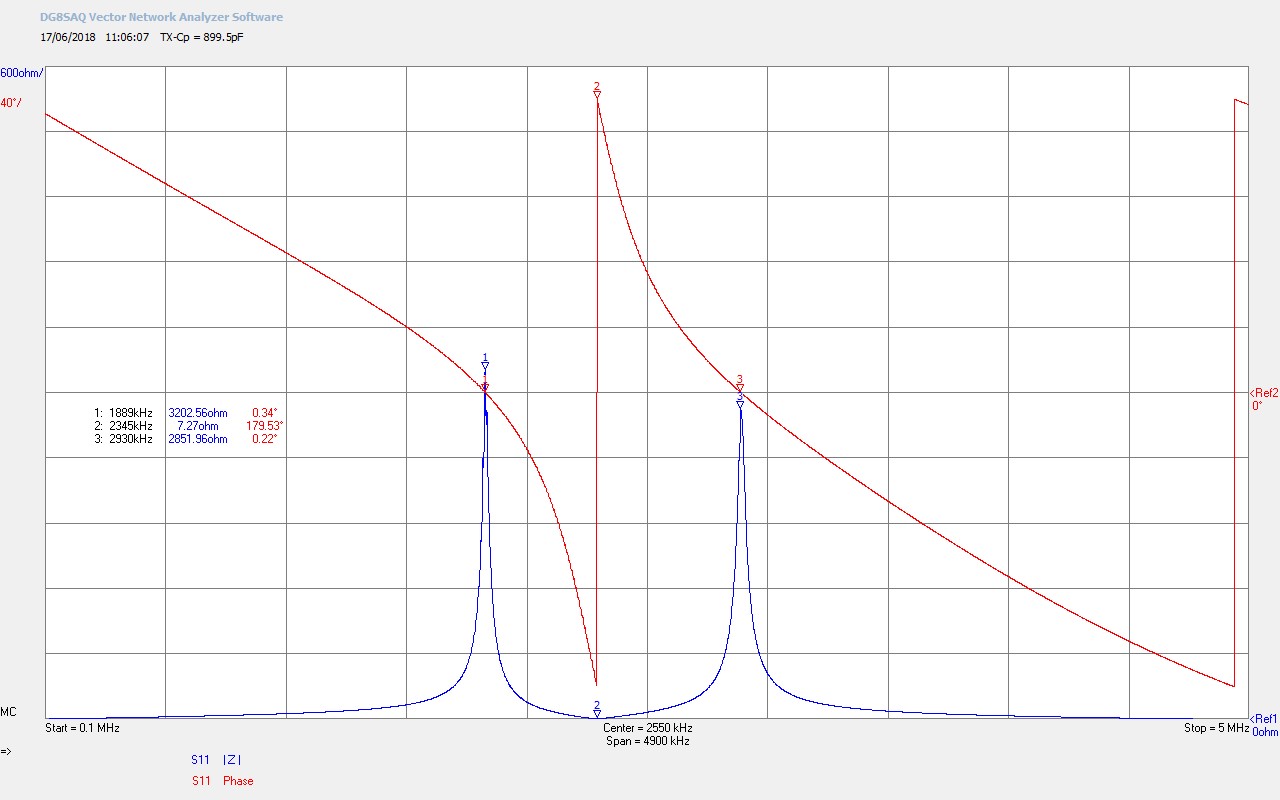
Fig. 4.1. Z11 input impedance as seen by the generator of the experimental setup including the matching unit, flat coil 1S-3P, RF meters, load bulbs, and measuring probes, and the single output wire connected to the load.
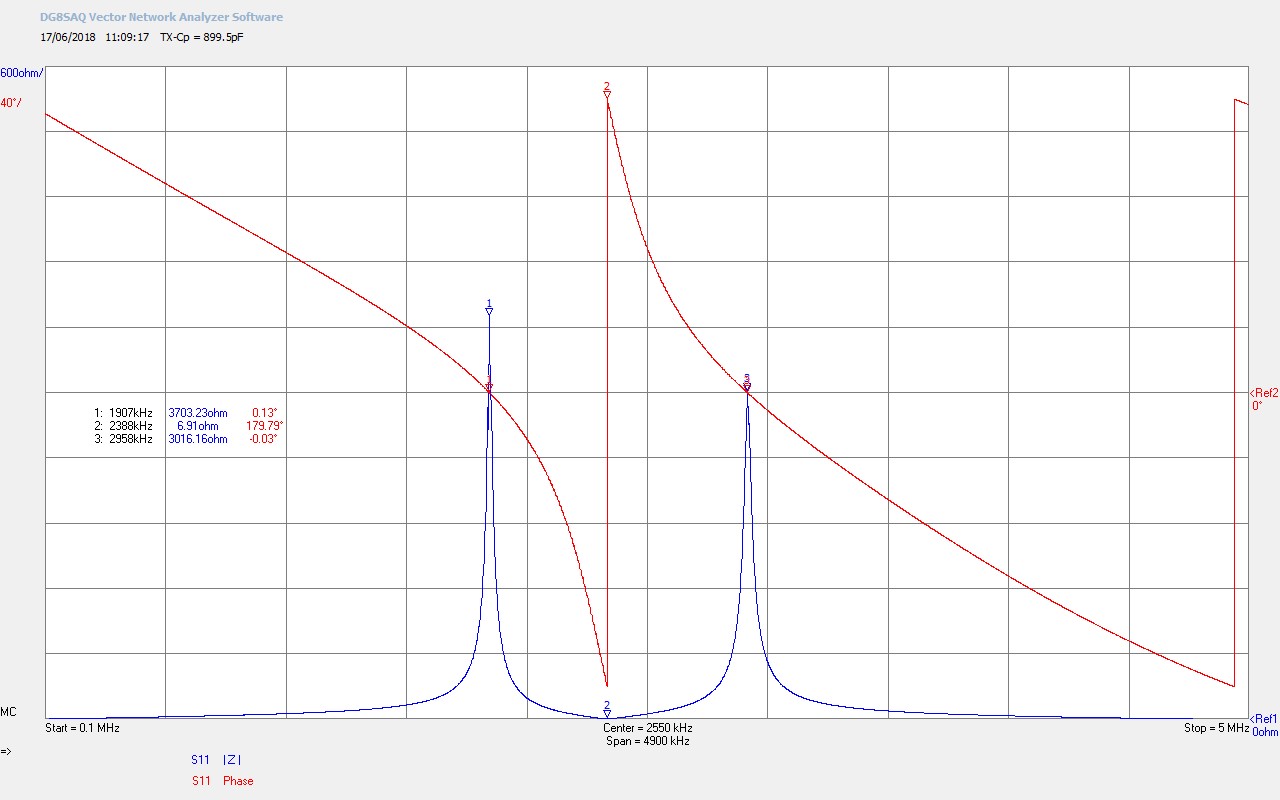
Fig. 4.2. Complete experimental setup with the single output wire disconnected from the load.
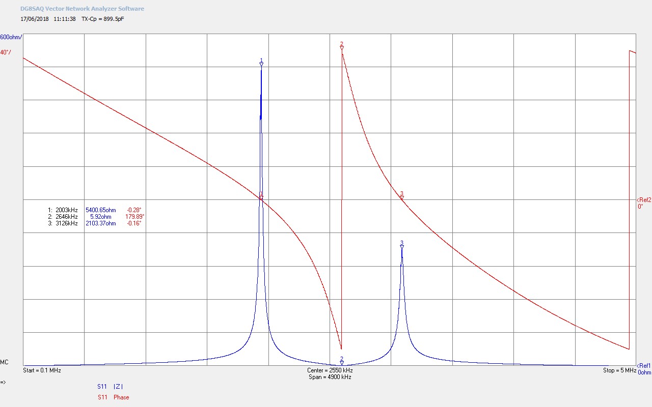
Fig. 4.3. Experimental setup with the bottom-end of the flat coil disconnected from the wire feeding the secondary rf meter, (meter, load, and probes disconnected).
Fig. 4.4. Complete experimental setup with the primary capacitor disconnected.
To view the large images in a new window whilst reading the explanations click on the figure numbers below:
Fig 4.1. Shows the small signal input impedance Z11 as seen by the generator of the complete experimental apparatus with all measurement probes connected, and the fly lead connected at the output of the bulb load. The impedance characteristics show that the experiment tuning is operating very close to the balanced point between the lower and upper resonant frequency, FL and FU, of the flat coil. This is the point where there is expected to be best balance between the electric and magnetic fields of induction between the primary and the secondary coils, and in this case the best experimental starting point when investigating the displacement and transference of electric power through non-linear processes. FL measured when running the single wire current experiments was ~1850kc/s, and from the impedance characteristics 1889kc/s a variation of ~2%, and most likely due to differences between the small-signal and large-signal operation points of the flat coil, tuning components, and generator mode of operation (cw class-C).
Fig 4.2. Shows the result of removing the fly lead the length of wire in the secondary section of the experiment has been reduced, and hence the frequency increased from ~1850kc/s to ~1860kc/s. This is also indicated by the impedance characteristics where the 180° phase change frequency FØ180 has shifted from 2345kc/s in Fig. 4.1 up to 2388kc/s. This has also created a greater imbalance between FL and FU.
Fig 4.3. Shows the result of removing the experiment from the bottom-end or outer-end of the secondary coil. All frequencies are shifted up due to the change again in wire length, and also the change of impedance at the bottom-end from lower to higher, and away from the λ/4 mode.
Fig 4.4. With the primary capacitance CP removed the impedance characteristics of the experiment revert to the loaded properties of the secondary coil with a single resonant frequency, and there is no established balance between the electric and magnetic fields of induction between the primary and the secondary.
Summary of the results and conclusions so far:
1. Single wire currents have been observed and measured using a flat coil driven by a vacuum tube generator in cw mode. The current measured in the single wire, and its properties thus far observed, would appear to suggest that rf energy from the wire is escaping along its length to the surrounding environment which acts as an energy sink, ground, or -ve terminal, which then effectively completes the circuit. High energy rf as a result of the magnified voltage produced by the secondary coil, is easily radiated from all parts of the conductor that forms the wire through to the end of the fly lead. With this being the case, and with the voltage and current being in phase in the secondary, real power is generated to drive the load bulbs which emit both light and heat. With the fly lead removed the final load bulbs do not light as there is insufficient length of conductor to act as a suitable radiator or sink “to ground”. It is expected that any load connected to the end of the single wire will not be driven as there is insufficient energy sink on the output of the load to enable a current to be developed through the load. With this being the case the energy sink is distributed along the length of the wire so that the current along the wire would not be a constant value, as might be expected normally for the current flowing through a circuit. In part 2 of single wire currents it will be necessary to measure the magnitude and phase of the current along the wire length as a function of distributed load which would then allow a more accurate picture, and hence interpretation, of single wire current action in a circuit.
2. Standing waves were not observed or measured along the length of the single wire in this experiment, but rather the magnitude of the oscillating voltage appears to remain relatively constant along the length of wire, whilst the current reduces with load and distance along the wire. This will be further investigated in part 2 where a more accurate voltage and current distribution will be measured with wire length and load distribution.
3. A force applied to a conductive medium in close proximity to a load on the wire, in this case a lighted incandescent bulb filament, has been observed and investigated at first stage. The phenomena, at this stage, appears to result from a form of electric attraction between the filament of the bulb the emitter, and the conductive medium. The effect does not appear to be influenced by other close proximity magnetic fields such as permanent magnets, and electromagnets, which also suggests that the phenomena does not result from eddy currents generated in the conductive medium. A range of different materials have been tested, and all that show a significant attraction towards the load bulb, have a conductive element or property. The effect is also greatly amplified in the presence of a significant energy sink such as the hand of a person. In cw mode no discernible force could be registered on the surface of the hand when placed in close proximity to a load bulb. This has been subsequently demonstrated when driving the generator in burst or impulse mode and will be presented in detail in subsequent parts.
4. The impedance characteristics indicate that the complete experiment was operated in a well-balanced mode of the flat coil, which suggests a good starting point for further, and more detailed investigation, of the displacement and transference of electric power through non-linear events.
Click here to continue to Transference of Electric Power – Part 1.
1. A & P Electronic Media, AMInnovations by Adrian Marsh, 2019, EMediaPress
2. Dollard, E. and Energetic Forum Members, Energetic Forum, 2008 onwards.
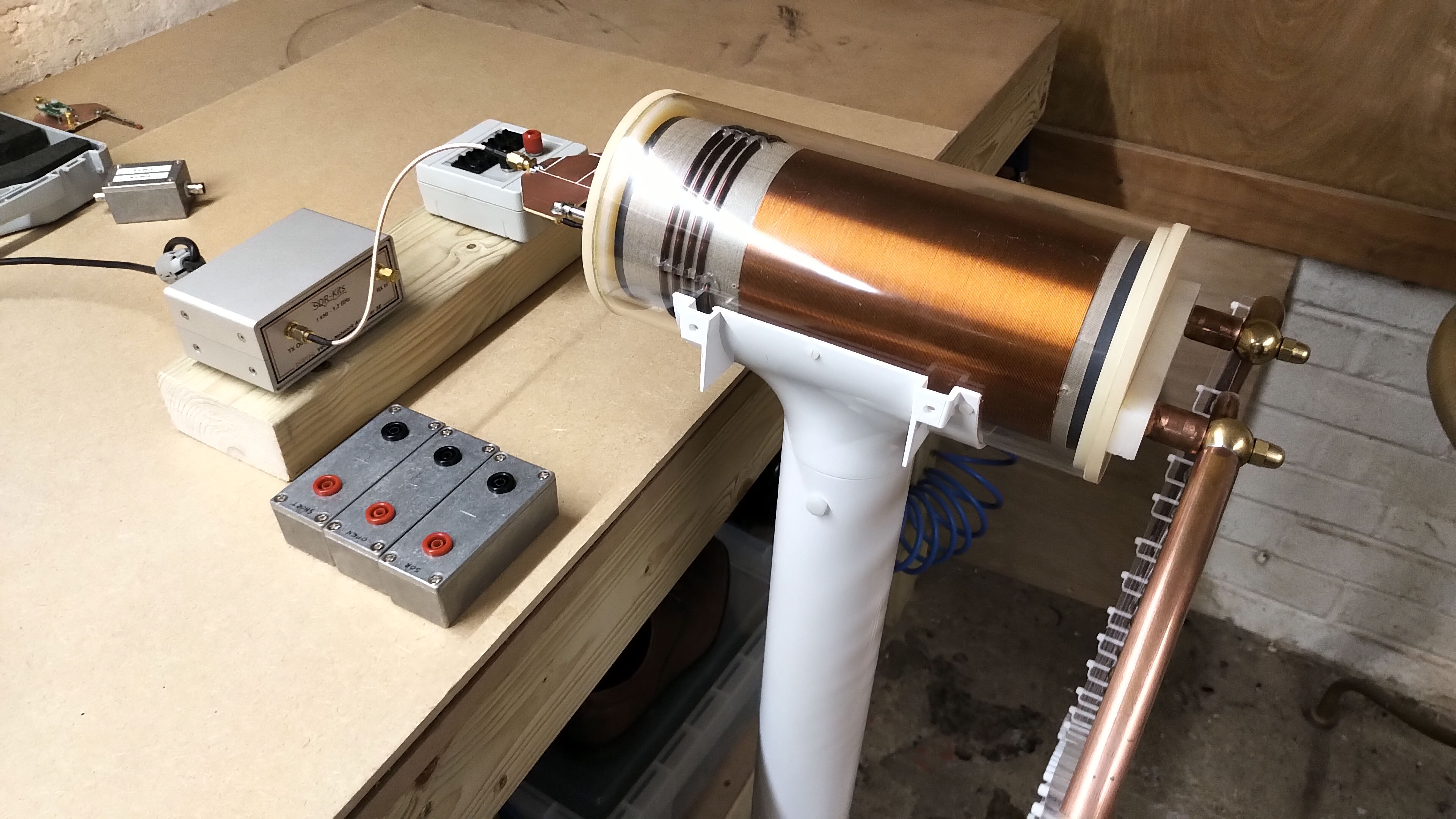
The original Lahkovsky Multiwave Oscillator (MWO) apparatus combines two Tesla style drive coils in a transmitter and receiver configuration, each consisting of a primary and secondary coil cylindrically mounted on axis. The top-load for both transmitter and receiver is a complex combination of concentric half-wave resonators. The impedance characteristics of even a single drive coil with top-load represents a complex measurement challenge with results that can span over a very wide frequency range, in the order of 100kc/s – > 1Gc/s.
In this first part the small signal impedance characteristics, Z11 (magnitude and phase) with frequency as seen by the generator, are measured for a single drive coil both with and without the MWO top-load over the lower frequency range of 100kc/s – 20Mc/s. In this measurement the impedance characteristics are dominated by the drive coil which will mask any higher frequency measurements pertaining to the MWO top-load. For this reason the top-load is measured individually in part 2 in the frequency range 100kc/s – 1.3Gc/s. Subsequent parts will look at the overall MWO system impedance characteristics when both transmitter and receiver are combined together in the original Lahkovsky arrangement, and later in an optimised and balanced drive arrangement as designed and presented by Dollard[1].
In this first part the following measurements are presented:
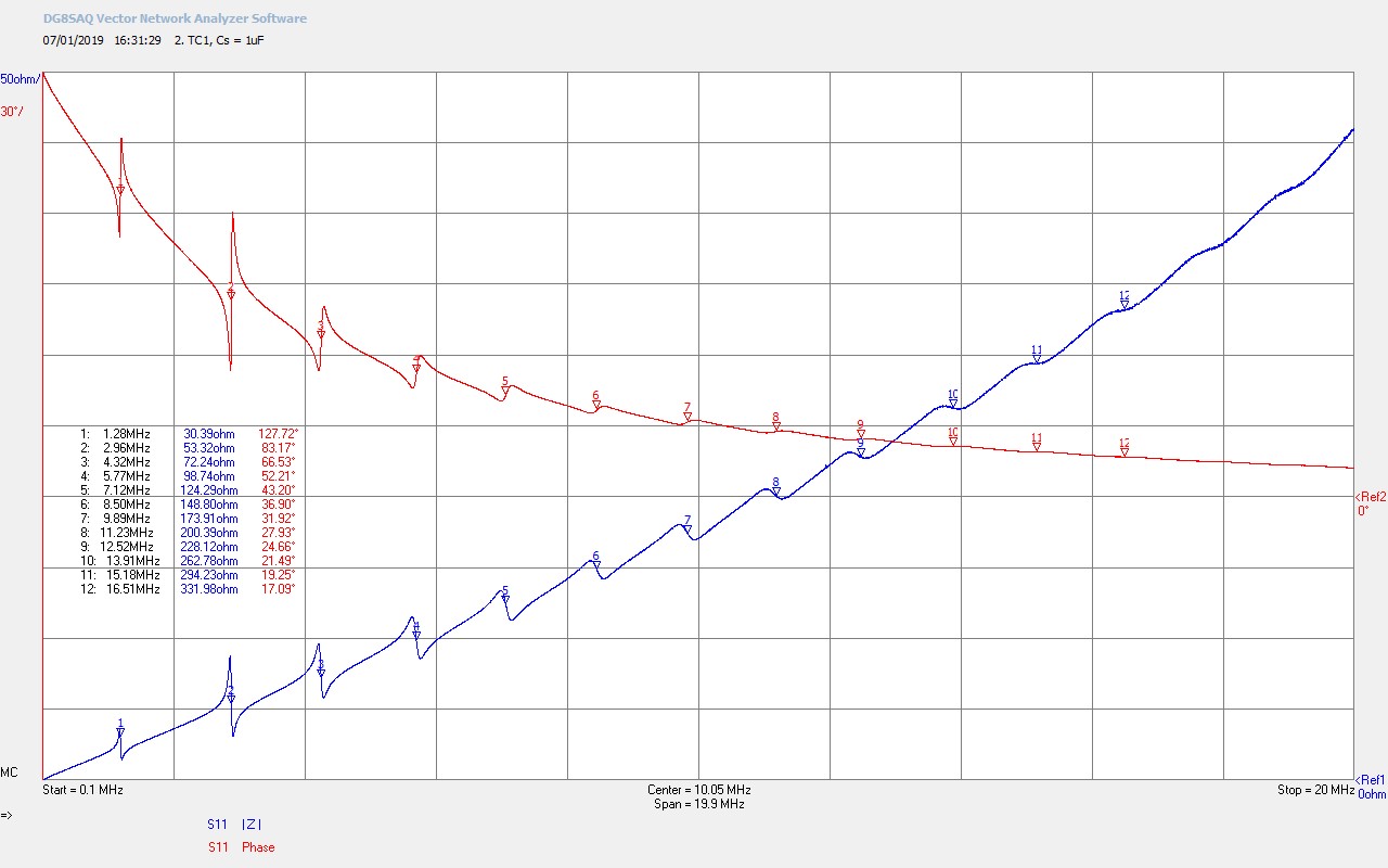
1. Z11 (magnitude and phase) with frequency for a drive coil without MWO top-load in the range 100kc/s – 20Mc/s
2. Z11 for the drive coil combined with MWO top-load, and over the same frequency band.
3. Primary tuning measurements to match the resonant frequency of the primary coil, (with series loaded Cp), to the secondary coil at the fundamental, second, and third harmonics.
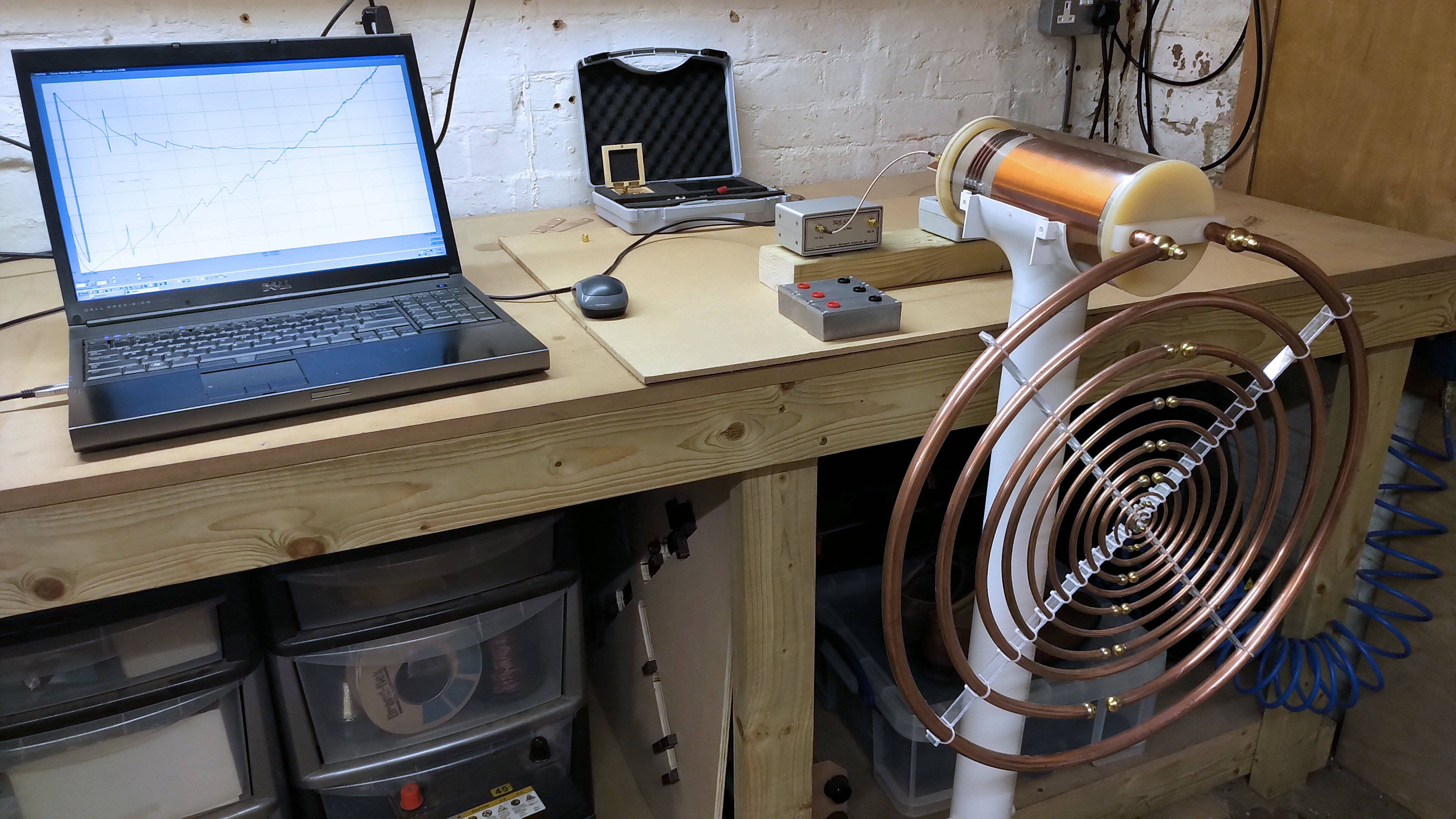
The SDR-Kits Vector Network Analyser 3E (VNA-SDR) was used to make all Z11 measurements, and the apparatus and method of measurement is shown in Figures 1 below.
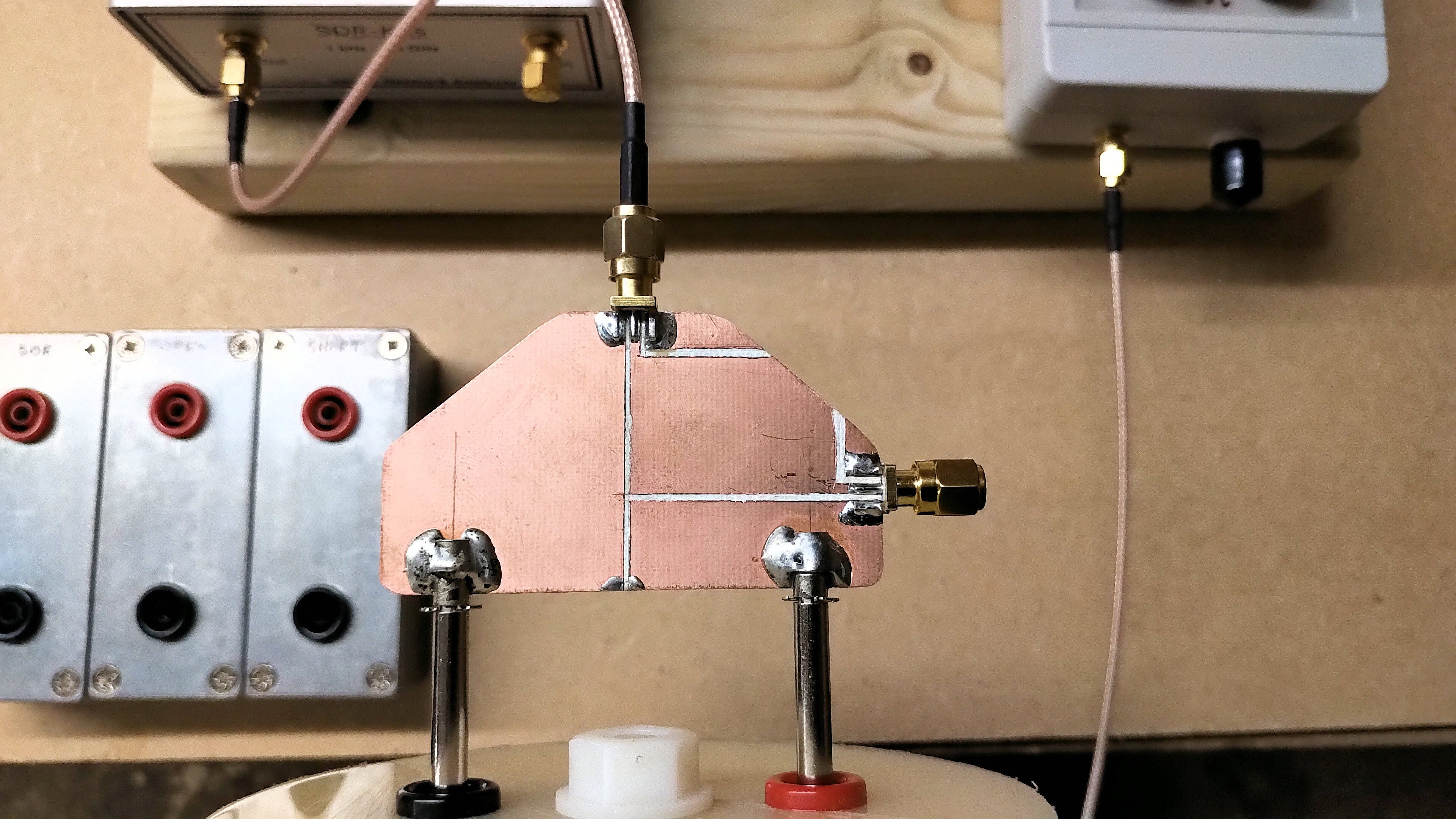
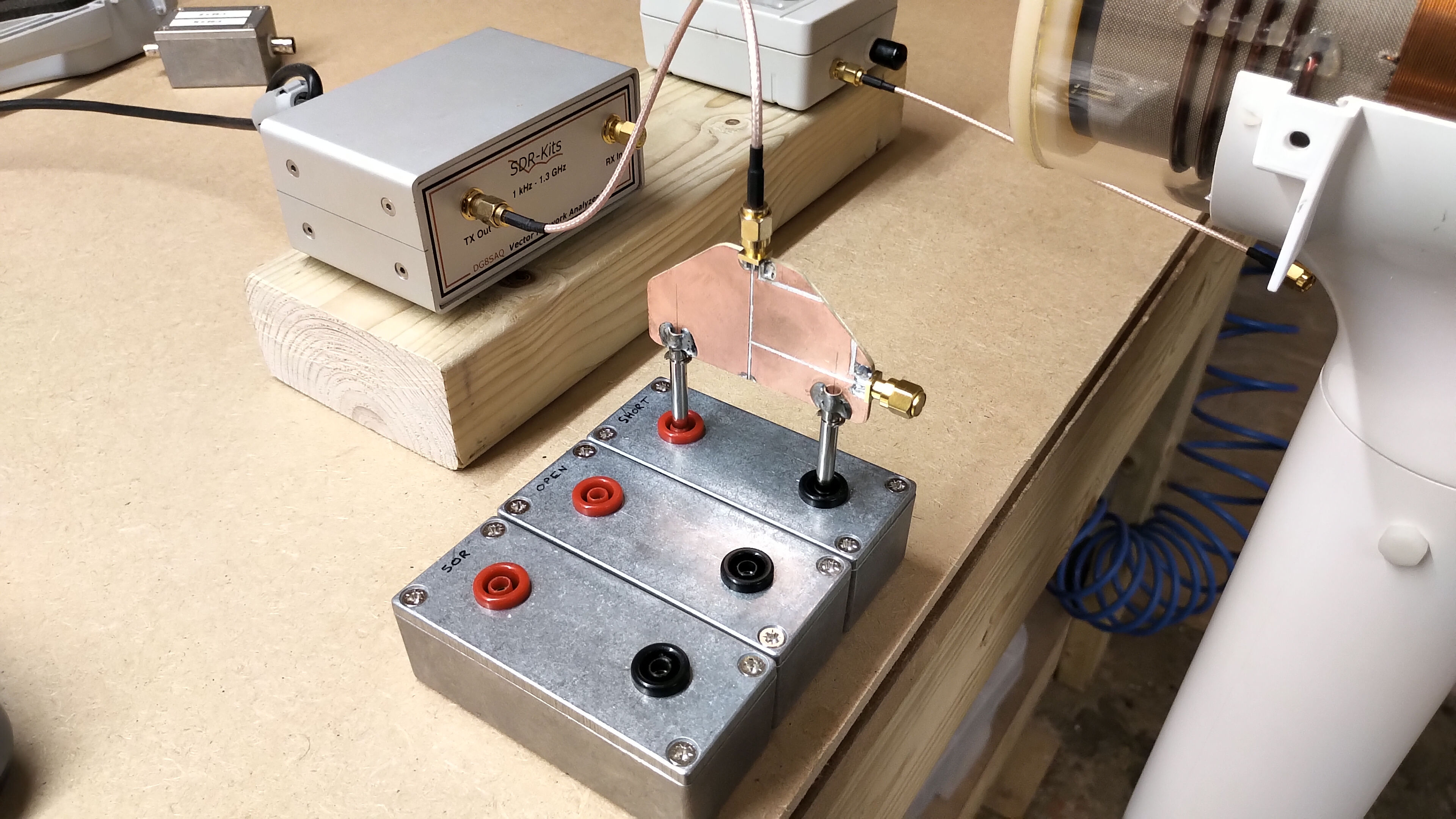
Fig. 1.1 Experimental setup for the MWO TC drive Z11 impedance measurements, showing the TC drive coil, VNWA-SDR, calibration modules, and connection to the computer.
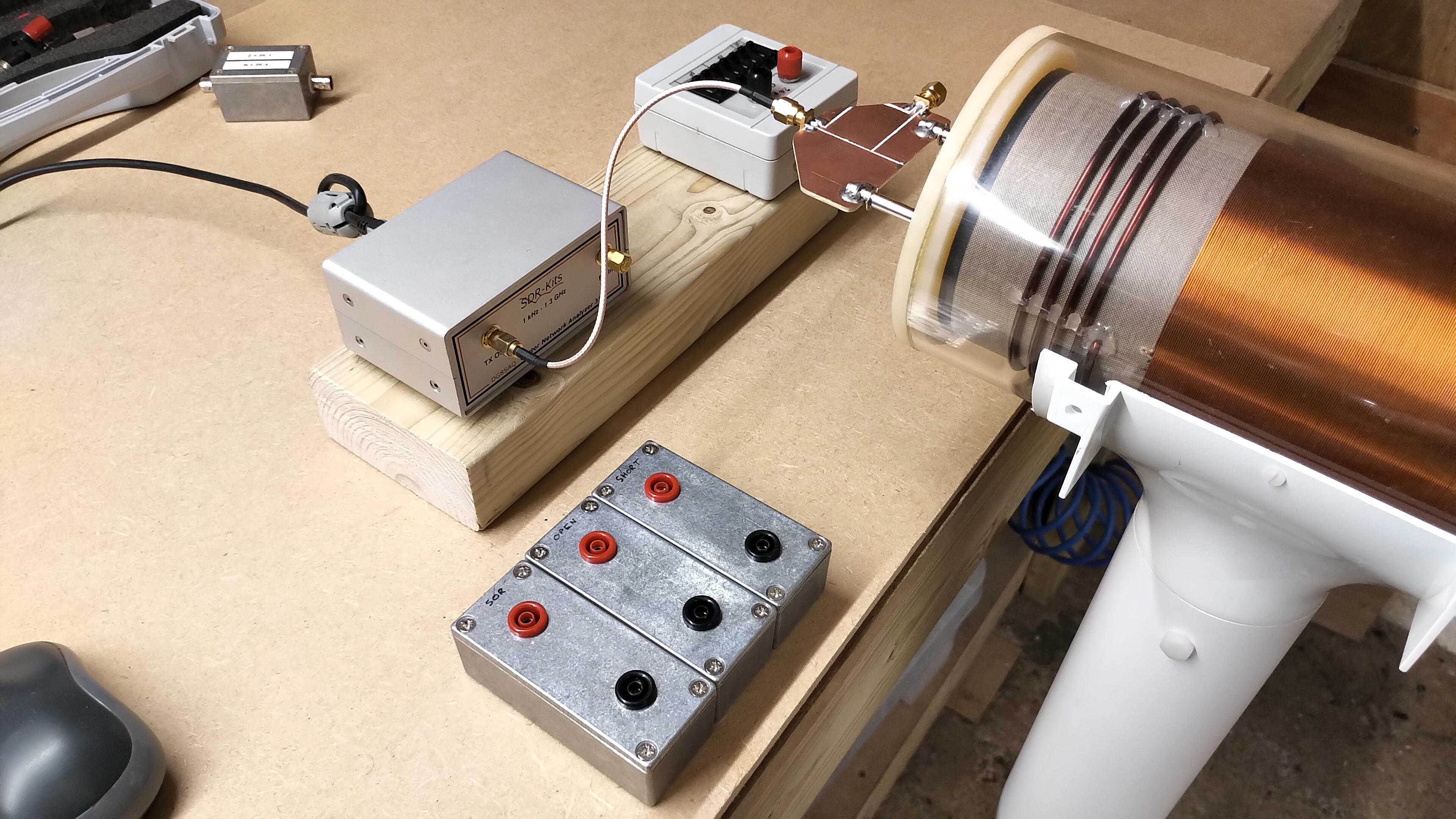
Fig. 1.2 The TC drive coil is connected via a pcb feed adapter to the VNWA-SDR via a short SMA RG178 coaxial cable.
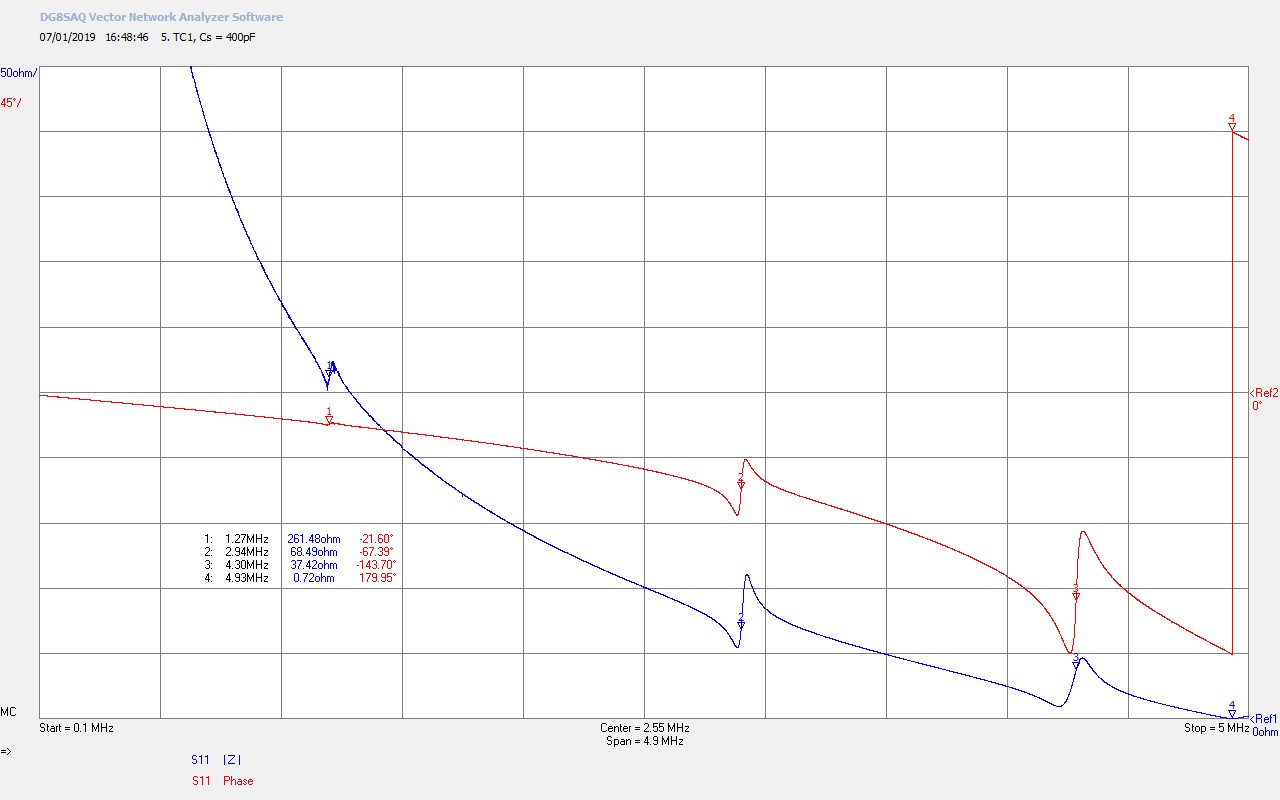
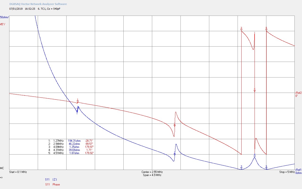
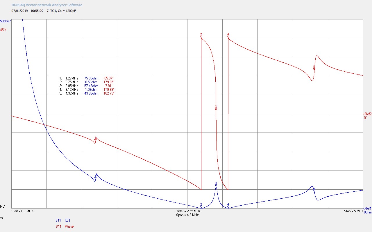
Fig. 1.3 The TC drive adapter pcb is arranged to feed the TC via an SMA connector which allows for a calibrated series capacitance to be connected, and hence different resonant tuning points between the primary and the secondary.
Fig. 1.4 The feed pcb enables the VNWA-SDR calibration to extend right to the input terminals of the TC, eliminating spurious measurement effects from the connectors, cables, and geometry.
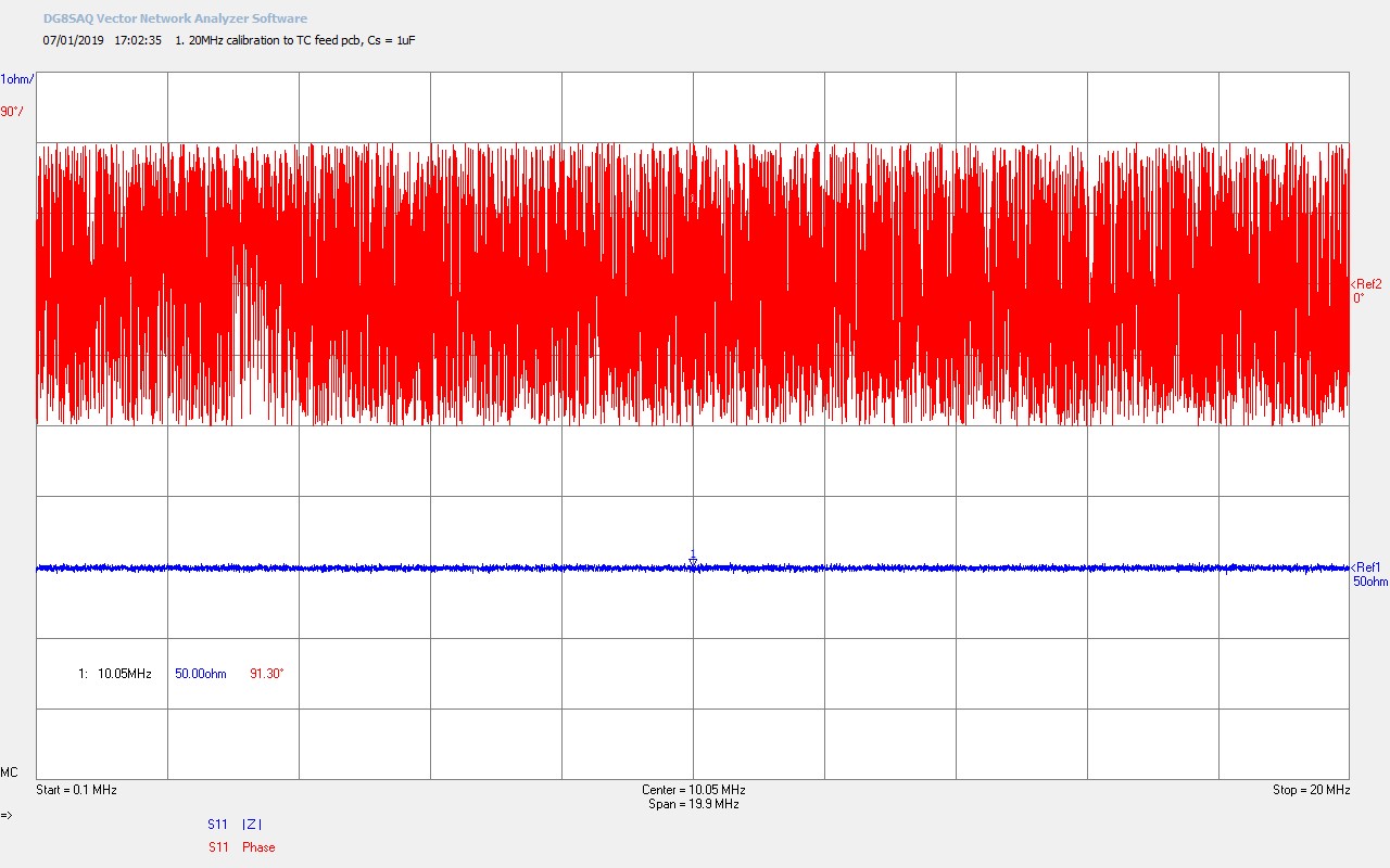
Fig. 1.5 The pcb feed adapter is calibrated in stages against a standard short circuit, open circuit, and 50Ω load. The series capacitance connector is here shorted with an SMA short when not being used.
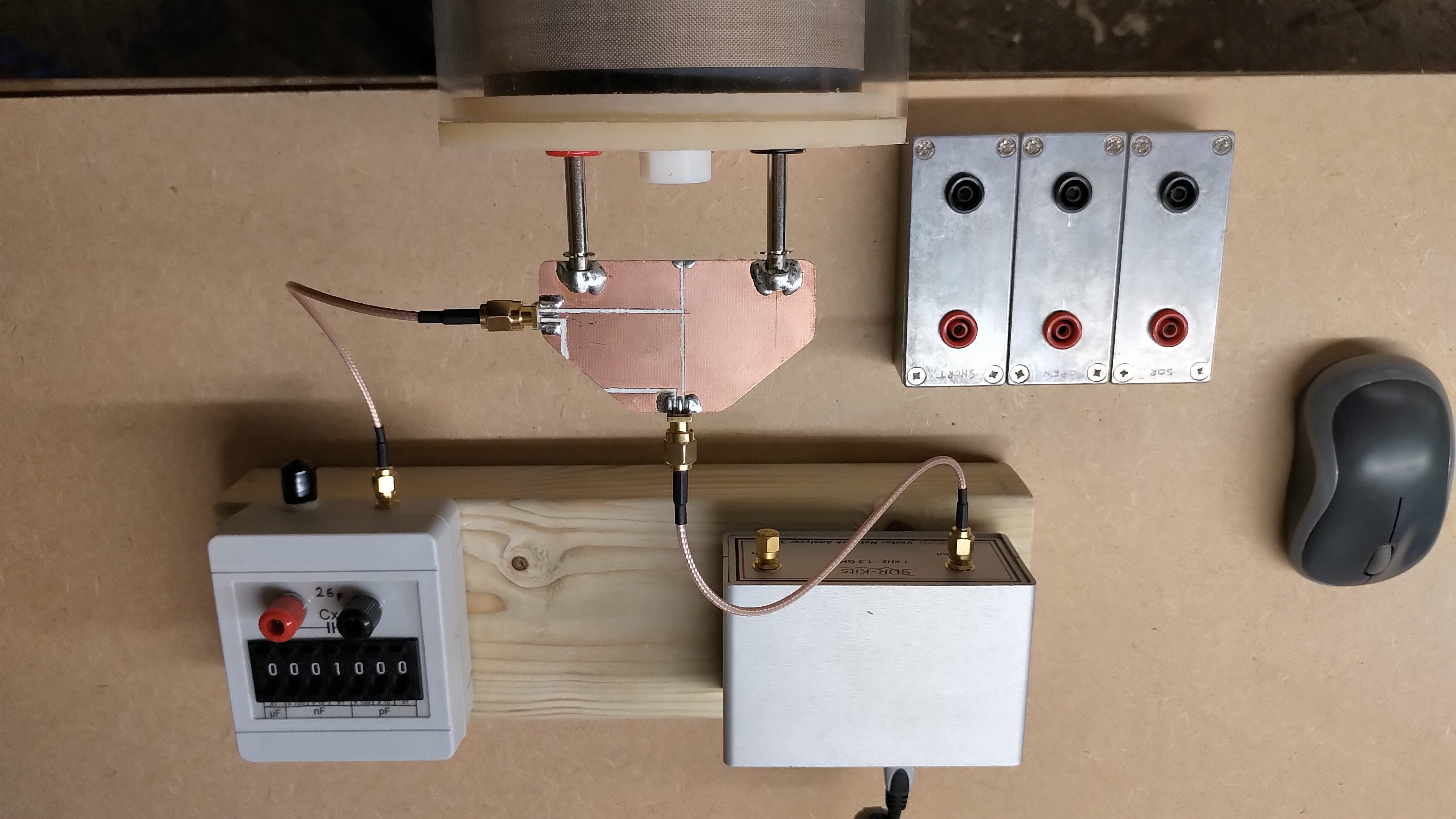
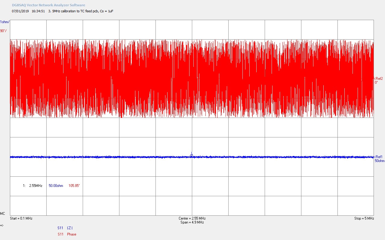
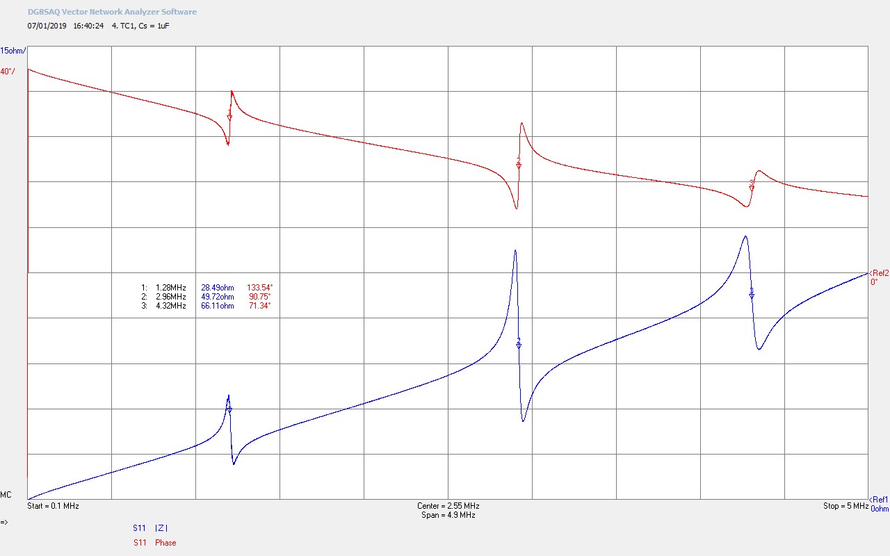
Fig. 1.6 Here the feed pcb is connected to both the VNWA-SDR and a calibrated series capacitance box Cs. With both connected the VNWA was first calibrated using the three standard loads with Cs set to 1uF.
Fig. 1.7 The TC drive coil connected with MWO topload and measured in the same way as before to compare the impedance loading effects.
Fig. 1.8 The MWO topload is connected directly to the TC drive coil via short copper spacers where one end is driven from the secondary coil output, and the other open circuit, forming a λ/4 or shorter driven outer ring.
To view the large images in a new window whilst reading the explanations click on the figure numbers below.
Fig 1.1. Shows the overall measurement setup with the VNA-SDR connected to the drive coil by a short SMA terminated RG316 cable, and the other end to the coil feed adapter, and standard calibration modules.
Fig 1.2. The drive coil used in these measurements has 4.5 primary turns of AWG 10 ~2.5mm diameter magnet wire, and the secondary has 248 turns of AWG 24 ~0.51mm diameter magnet wire. The top-end of the primary coil is connected directly to the bottom-end of the secondary coil and forms the negative or ground terminal. The positive or drive terminal is connected to the bottom-end of the primary coil, and the top-end of the secondary can be seen emerging from the coil through a brass bolt which attaches to the driven top-load. Both coils are wound anti-clockwise on the former from the base.
Fig 1.3. In order to make an accurate measurement of Z11 it is necessary to calibrate the VNA-SDR as close to the drive coil as possible. In this case the calibration plane is extended to the input of the primary coil terminals, (two 4mm high voltage shielded terminals), via a signal feed adapter pcb (SFA). The SFA can be removed from the drive coil by drawing the two-pronged 4mm probes out of the drive coil terminals. With the SFA disconnected the VNA-SDR can be calibrated by fitting an open, short and 50Ω standard load to the end of the SFA. The effective calibration plane then becomes the input to the drive coil, and spurious impedance effects due to any cables and the SFA itself can be removed from the final results. When calibrated, a frequency scan of the SFA with the 50Ω standard load will show a flat impedance line for |Z|, (magnitude of the impedance). The phase of this scan will swing repeatedly between ±180° indicating the near perfect match between the calibration plane and the 50Ω standard load.
Fig 1.4. Shows a close-up of the SFA connected directly to the two high voltage drive terminals in the base of the drive coil. The SFA has an SMA input feed and is then connected via equal weights of copper to the series connection point. The black terminal indicates the negative or ground point where both primary and secondary are connected together, and the red terminal the high voltage feed end of the primary. The series connection point in the positive terminal allows for a calibrated capacitance box to be connected in the primary circuit for tuning measurements. In this picture the series connection is not being used and is terminated with a SMA short. In tuning measurements, when series capacitance CS is added, the SFA must first be calibrated with the capacitance box connected to the SFA with a nominal 1µF set at its output. The 1µF series capacitance has a very low impedance at the measurement band of interest and acts effectively as a short-circuit of the series connector during the calibration procedure. During tuning measurements the capacitance of the box is reduced in the range 100pF – ~ 50nF. The capacitance box itself uses surface mount standard capacitance values and can be reasonably used with SMA connection up to ~ 100Mc/s. The SFA is an unbalanced feed adapter and takes an unbalanced coaxial cable input directly to a balanced two terminal output without any compensation for this change in balance. A similar SFA was also tried which incorporated an RF (upto ~ 3Gc/s) balun in order to effect the transformation between the unbalanced and balanced connections. However, even with calibration the balun SFA proved to be less effective to measure Z11 accurately and cleanly, as it dominated the impedance changes in the frequency band masking changes due to the drive coil further downstream. The standard SFA was therefore used with careful calibration up to the intended reference plane at the input terminals to the coil.
Fig 1.5. Shows the calibration procedure where the SFA is connected in turn to the standard calibration modules, here connected to the short circuit module. In this case the series capacitance terminal is not being used and is shunted with an SMA short.
Fig 1.6. Shows the SFA in measurement configuration and after calibration, where a 1nF series capacitance is added to the primary feed. The calibrated capacitance box can be adjusted in 1pF increments in the range ~30.5pF – ~10µF, where the parasitic capacitance of the box with SMA cable and when set to zero is ~30.5pF.
Fig 1.7. Shows the overall measurement setup with the top-load connected, and then calibrated and measured in the same procedure as previously discussed. The outer ring of the top-load forms an effective wire extension and capacitive load to the top of the secondary coil, which will both reduce considerably the fundamental resonant frequency and Q-factor of the drive coil. When compared with the drive coil without top-load the outer ring forms a λ/4 driven ring, which is coupling to 11 other λ/2 resonating rings. Given the size of the outer driven ring, and the proximity of the inner rings the coupling factor is considered to be quite high between the driven ring and the inner resonators, which will tend to constrain the free resonation of the inner rings and considerably quench the Q and hence measurements at much higher frequency. This is considered more closely in part 2.
Fig 1.8. Shows in more detail the mounting points at the top-end of the secondary and the MWO top-load.
Figures 2 below show the Z11 impedance characteristics of the calibrated reference plane, the drive coil, and primary and secondary tuning with series added capacitance, of the drive coil only.
Fig. 2.1 Calibration results for the 50Ω standard load over the measurement window of 100kc/s - 20Mc/s. This calibration takes into account the TC feed pcb and a series capacitance Cs = 1uF, creating a calibrated reference plane at the TC input connectors.
Fig. 2.2 Magnitude and phase for Z11 showing the fundamental resonant frequency of the TC at M1 (1.28Mc/s), and many harmonics, (the VNWA-SDR software allows for a maximum of 12 simultaneous marker points).
Fig. 2.3 Narrowband calibration for Z11 against the 50Ω module over the range 100kc/s to 5Mc/s, to measure with greater detail the fundamental resonant frequency, 2nd, and 3rd harmonics.
Fig. 2.4 The fundamental resonant frequency, 2nd, and 3rd harmonic for the TC drive with a series primary capacitance Cs = 1uF, (very low impedance across the band).
Fig. 2.5 The series capacitance in the primary reduced to 400pF to show the 180° phase change in the primary that occurs at resonance (M4), and the accompanying very low series resistance at resonance.
Fig. 2.6 Cs has been increased to 540pF where the resonant frequency in the primary matches the resonant frequency of the 3rd harmonic of the secondary at M4 (4.31Mc/s). The matched primary and secondary resonance cause frequency splitting in Z11 at M3 and M5.
Fig. 2.7 Cs is further increased to 1200pF where the primary and secondary match now occurs at the 2nd harmonic M3 (2.95Mc/s).
Fig. 2.8 The primary and secondary resonance now match at the fundamental resonant frequency at M2 (1.28Mc/s), and Cs = 6500pF. When driven by a non-linear generator such as a spark gap the primary would resonate predominately at M1 (1.17Mc/s) with many other harmonics and beat frequencies present.
Fig 2.1. Shows the calibrated reference plane of the SFA when connected to the 50Ω standard load over the wideband range 100kc/s – 20Mc/s. The calibration is as expected and accurate over the band, with a slight phase variation between ~ 3 – 3.5Mc/s indicating a resonance in the signal path between the calibration plane and the VNA-SDR which has been normalised out by the calibration procedure.
Fig 2.2. The impedance characteristics of the drive coil with the series capacitance Cs = 1µF, showing a wealth of resonant peaks and corresponding phase changes from the fundamental resonant frequency FS of the secondary coil at 1.28Mc/s up to the 12th harmonic FS12 (M12) at 16.51Mc/s. It is interesting to note that the 2nd harmonic FS2 at M2 is a stronger resonance than that of the fundamental at M1. This is further demonstrated in subsequent impedance results. The VNA-SDR allows for only 12 concurrent markers which is why the final two harmonics on the results are not marked. At frequencies above 20Mc/s the rapidly increasing inductive impedance of the primary masks out any further harmonic points of interest, and the impedance curve rises rapidly until the primary coil becomes self-resonant at ~38Mc/s.
Fig 2.3. Shows the calibrated reference plane of the SFA when connected to the 50Ω standard load over the narrowband range 100kc/s – 5Mc/s. With more accurate calibration in the narrowband it can be noted that the phase variation seen in Fig. 2.1 has now been completely normalised out of the reference plane.
Fig 2.4. Shows the narrowband impedance characteristics for the fundamental FS and the first two harmonics FS2 and FS3. Here the difference in magnitude of the resonance between FS and FS2 can be very clearly observed, although the Q of the coil remains very similar for both frequency points. The magnitude of the impedance |Z11| ~ 28.5Ω at FS, and ~ 49.7Ω at FS2 would significantly impede currents developed in the primary from the generator, coupling very little power to the secondary and ultimately to the MWO top-load. The primary circuit will need to be brought into resonance with the secondary at the corresponding frequency in order to considerably reduce the driving impedance seen by the generator, and hence maximise the primary currents, and the amount of power transferred from the generator through the drive coils to the top-load. On the very far left of the scan at 100kc/s the 180° phase change FØ180 of the primary in resonance with the series capacitance CS can just be observed. This will be adjusted by varying CS in subsequent results in order to tune the primary resonant frequency to that of the secondary. Given the difference in magnitude between the fundamental at FS and the 2nd harmonic at FS2 it may be more optimal to arrange the primary to resonate at FS2 rather than the fundamental for normal experimental operation. This will be tested during experiments and reported in subsequent parts.
Fig 2.5. Here the series capacitance CS has been reduced from 1µF to 400pF which has increased FØ180 (the resonant frequency of the primary to M4 at 4.93Mc/s. At this point the impedance seen by the generator has reduced drastically to ~0.72Ω allowing for much larger primary currents. In this case FØ180 does not correspond to a resonant frequency in the secondary so reduced power would be transferred between the two coils. At lower frequencies in the measurement band, the impedance of CS is higher and has the effect of attenuating currents in the primary reducing considerably the magnitude of the lower resonant points, in this case considerably suppressing the fundamental resonance at FS. This scan clearly shows the effect of including a series resistance in the primary and making it resonant within the measurement band of interest.
Fig 2.6. Here CS has been increased to 540pF which has brought the resonant frequency of the primary equal to the 3rd harmonic resonance of the secondary at M4 at 4.31Mc/s. As always with coupled resonant circuits, mixing of the signals causes beat frequencies and hence frequency splitting into two sideband frequencies where the impedance minimum points are at both the lower and upper resonant frequencies FL3 (M3) and FU3 (M5) respectively. If driven by a generator with CS = 540pF FL3 would be the best driving point since proximity coupling to the secondary top-load, or discharge of stored energy on the top-load, would momentarily increase the loading on the coil reducing slightly its secondary harmonic frequency towards FL3, and hence maximising transference of electric power between the primary and secondary coils.
Fig 2.7. Shows CS increased further to 1200pF which now tunes the primary resonance to the 2nd harmonic FS2 at M3 a frequency of 2.95Mc/s. Again frequency splitting occurs and the impedance of FL2 and FU2 are very low ~0.5 – 1Ω facilitating high current drive from the generator.
Fig 2.8. Shows CS finally increased to 6500pF which tunes the primary to the fundamental resonant frequency of the secondary FS at M2 at 1.28Mc/s. At FL (M1) the lowest impedance drive point is obtained of just 0.34Ω at 1.17Mc/s. Given the very similar minimum |Z| characteristics of both FS and FS2, when tuned respectively to the primary with corresponding values of CS, either the fundamental or 2nd harmonic could be used to operate the coil in experiments to explore MWO operation and effects.
Figures 3 below show the Z11 impedance characteristics of the calibrated reference plane, the drive coil, and the primary and secondary tuning with series added capacitance, of the drive coil with the MWO top-load.
Fig. 3.1 Same wideband Z11 impedance characteristics for the TC drive now including the MWO topload. The fundamental M1 has moved down significantly from 1.28Mc/s to 650kc/s and is also quite strongly suppressed. The 2nd harmonic has strengthened, and the other higher harmonics remain mostly unchanged.
Fig. 3.2 Narrowband detailed impedance scan for the fundamental resonant frequency, 2nd, and 3rd harmonics.
Fig. 3.3 Cs = 400pF which represents a higher impedance at lower frequencies, and almost entirely suppressing the fundamental resonance.
Fig. 3.4 Cs = 570pF a slight increase, (previously 540pF without the MWO), in series capacitance in the primary in order to match the primary resonance with the secondary 3rd harmonic.
Fig. 3.5 Cs = 1300pF again a slight increase, (previously 1200pF without the MWO), in series capacitance in the primary in order to match the primary resonance with the secondary 2nd harmonic.
Fig. 3.6 Cs = 26000pF a very large increase, (previously 6500pF without the MWO), in series capacitance in the primary in order to match the primary resonance with the secondary fundamental.
Fig 3.1. Shows the wideband scan for the drive coil with MWO top-load on the same horizontal and vertical scaling as in Figures 2. The top-load at lower frequencies represents a considerable capacitive load at the top of the coil, very similar capacitively to a toroidal, cylindrical, spherical, or sheet metal top-load added to a conventional Tesla coil apparatus. The frequency of this scan is too low to show any of the high frequency features that result from the resonant rings of the MWO, (see part 2 for these features), but the capacitive loading of the MWO top-load could be clearly seen in this lower frequency scan. The biggest effect is noted at M1 at FS1 the fundamental resonance of the secondary which has reduced from 1.28Mc/s to 650kc/s, a 49.2% reduction . The 2nd and 3rd harmonics at FS2 and FS3 respectively have also reduced but in a much smaller range than the fundamental. FS2 has reduced from 2.96Mc/s to 2.84Mc/s a 4.1% reduction, and FS3 from 4.32Mc/s to 4.21Mc/s a 2.5% reduction. Higher harmonics also reduce with progressively reducing amounts up to FS12 at M12 which reduces from 16.51Mc/s to 16.46Mc/s a 0.3% reduction. It can be seen for this arrangement of drive coil the fundamental resonant frequency would be very sensitive and easily effected by metal loading to the top end of the secondary, the close proximity of metallic structures, or even to the proximity of partially conducting mediums such as the human body.
Fig 3.2. The narrowband scan shows the large change in the fundamental in relation to the 2nd harmonic both in frequency shift and in the magnitude of the impedance and phase change. The MWO top-load has considerably quenched the fundamental of the drive coil, whilst leaving the 2nd harmonic very similar to the coil only results (Figures 2) both in frequency and the magnitude of the impedance and phase.
Fig 3.3. Series capacitance CS = 400pF as before shows the primary resonance in the band, but in this case has completely quenched the already weak fundamental resonance. It can be seen that driving the MWO at the 2nd harmonic during experiments and operation may lead to considerably more stable and reliable system characteristics.
Fig 3.4. Shows the primary tuned at FS3 at M4 at 4.20Mc/s and a slightly increased series capacitance required to tune, increased from 540pF to 570pF.
Fig 3.5. Shows the primary tuned at FS2 at M3 at 2.83Mc/s and again a slightly increased series capacitance required to tune, increased from 1200pF to 1300pF. It can be noted that the fundamental resonance FS can now just be discerned at M1 at 650kc/s.
Fig 3.6. Shows the primary tuned at FS at M2 at 0.65Mc/s with FL = 610kc/s and FU = 700kc/s. The primary is tuned when CS = 26000pF (26nF) which is a very large increase on the 6500pF required without the MWO top-load. At FL (M1) the impedance seen by the generator in the primary is now 0.61Ω which is no-longer the lowest driving impedance. With CS = 1300pF and tuned to FS2 the driving impedance at FL2 is 0.47Ω which indicates that better power transfer from the generator to the secondary could be effected by driving the MWO at the 2nd harmonic. At this point the system would also be more stable and less effected by proximity of metal structures and other partially conductive mediums including the human body.
The lower frequency impedance measurements have shown a wealth of frequency harmonics associated with the Tesla style drive coil, and can be tuned progressively with the primary of the drive coil via series capacitance to make use of the system at different designed resonant frequency points. The MWO top-load at lower frequencies introduces a considerable capacitive load on the drive coil which has a large quenching effect on the fundamental resonant frequency of the system, and suggests a shift of optimal setup away from being driven at the fundamental and towards the 2nd harmonic where greater transference of electric power should be possible, and the system would be more stable and tolerant of loading conditions on the drive coils, the MWO top-load directly, and also from proximity of other conducting and partially conducting mediums. It will be interesting to determine if this changes when both the transmitter and receiver are combined in the full Lahkovsky MWO system, and also whether these effects can be directly demonstrated through experiments in the operation of the complete MWO system.
Click here to continue to part 2 of the multiwave oscillator impedance measurements.
1. Dollard, E., Design and presentation of an optimised and balanced MWO power supply and drive coils., Energy, Science, and Technology Conference (ESTC), 2018.