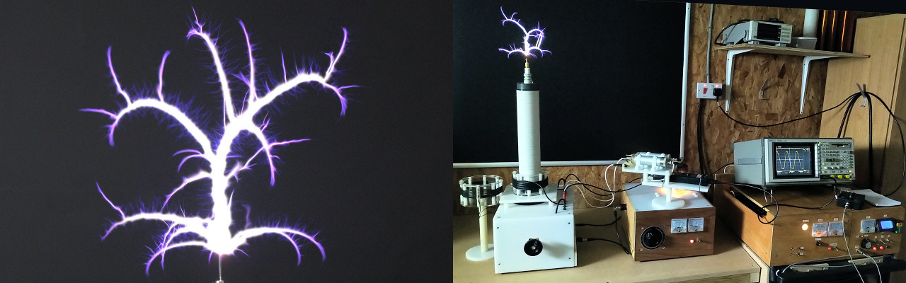
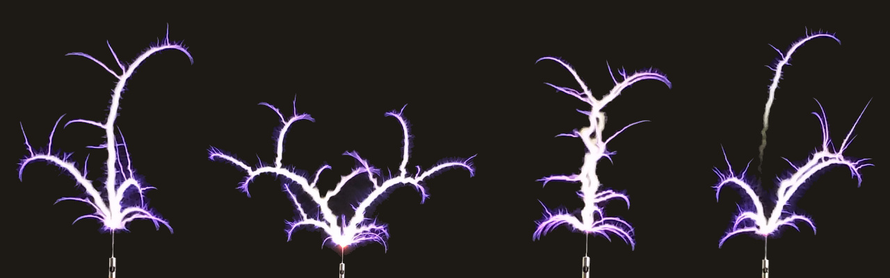
The Golden Ratio Discharge a fundamental part of The Wheelwork of Nature, revealing the underlying natural order expressed within electricity. (Click to enlarge images, and hover to pause slides)
The Golden Ratio Discharge showing well defined order, symmetry, as well as spatial and temporal coherence and choreography.
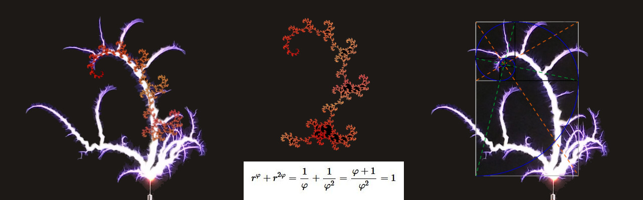
The Golden Ratio Discharge, also known as The Fractal-Fern Discharge, has its best fit in the form of The Golden Dragon, which is a fractal that expands according to the Golden Ratio.
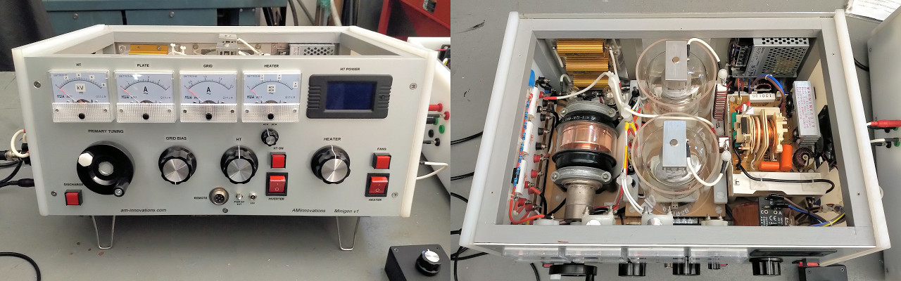
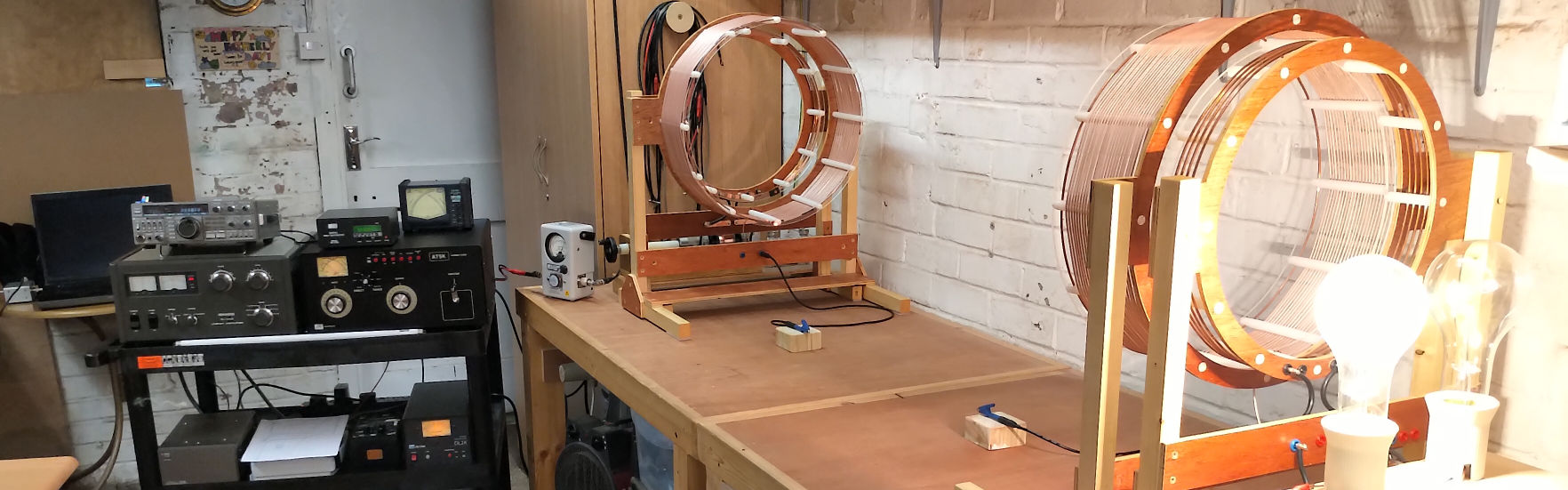
The AMInnovations MiniGen is a complete portable vacuum tube Tesla coil generator, and suitable for a wide range of different electricity experiments and demonstrations.
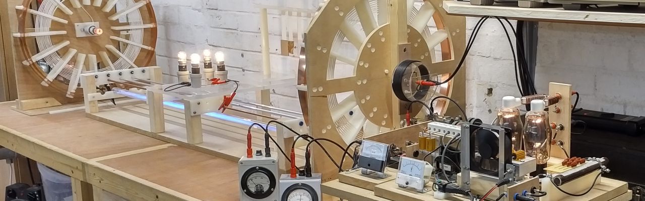
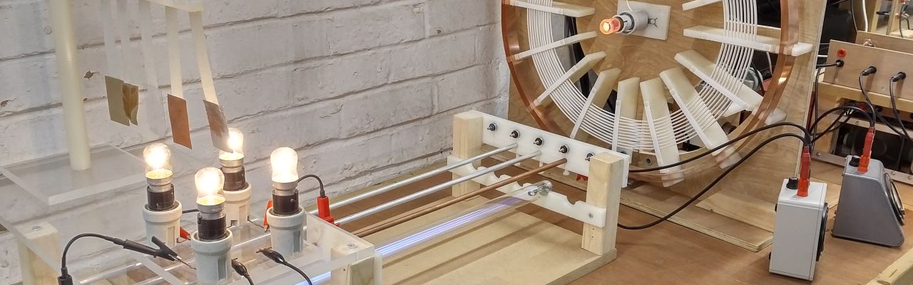
High-Efficency Transference of Electric Power experiments passing 500W of power across a 40awg (80 micron) single wire at an efficiency over 99.5%.
Plasma discharge, induction, and tension experiments using specialised Tesla Transformers driven by a vacuum tube generator, and similar in design to Eric Dollard's cosmic induction generator.
Experiments in the Displacement and Transference of Electric Power, using a flat-coil Tesla Magnifying Transmitter based on the design of Eric Dollard, Peter Lindemann, and Tom Brown.
A potential Radiant Energy event - a conjectured emission from Coherent Displacement in the single wire cavity of a Tesla Magnifying Transmitter with non-linear generator drive.
Displacement of Electric Power experiments using a high-energy discharge apparatus to explore non-linear displacement and disruptive phenomena, including "exploding wires", dielectric shock waves, and Tesla Radiant Energy emissions.
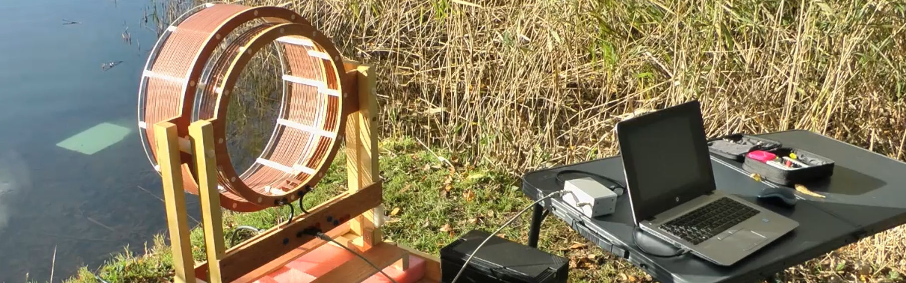
Telluric Transference of Electric Power experiments using a specialised Tesla Magnifying Transmitter, and measuring the proportion of telluric to radio-wave reception over 100 miles from the transmitter.
Telluric transference of electric power experiments using both two-coil and three-coil systems. The three-coil system includes Tesla's extra coil and introduces a more complex longitudinal cavity arrangement.
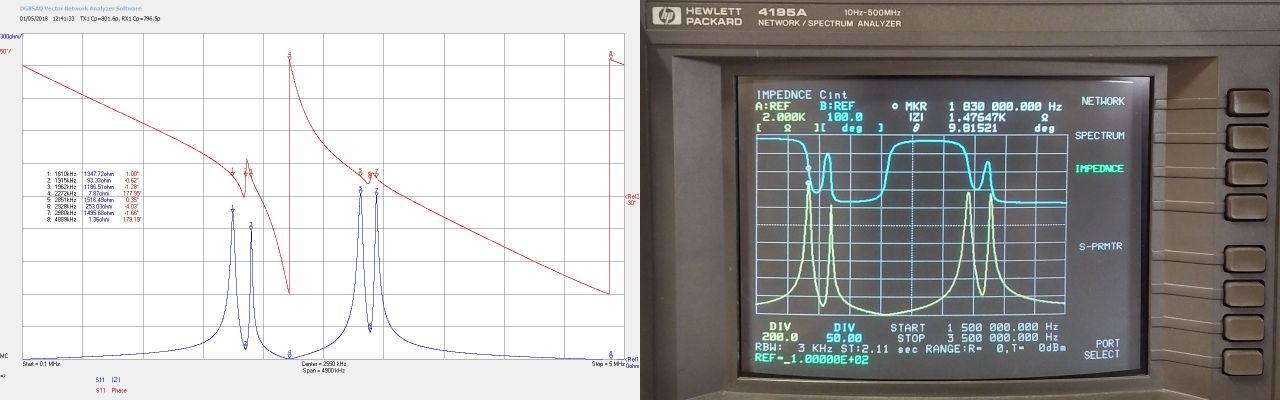
Input impedance Z11, as seen by the generator, of two flat coils bottom-end connected via a single wire cavity in a Tesla Magnifying Transmitter, and tuned to balance the Transverse and Longitudinal modes.
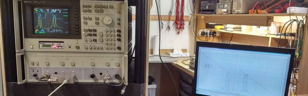
Input impedance frequency measurements of the twin coil experimental apparatus compared on a HP4195A and a SDR-Kits DG8SAQ VNA
Measured upper resonant frequency of oscillation for the single flat coil in Telluric electric power transmission tests.
"Electric power is everywhere present in unlimited quantities ...""Electric power is everywhere present in unlimited quantities and can drive the world's machinery without the need of coal, oil, gas ...""Electric power is everywhere present in unlimited quantities and can drive the world's machinery without the need of coal, oil, gas, or any other of the common fuels."Nikola Tesla c. 1900
In the early days of my research, and before we built the spark gap generator, it was unclear to me which parts of the electrical system were most directly responsible for generating unusual electrical phenomena, whether it be the generator or high voltage source, the types and arrangements of the various coils, or a combination of these elements setup and arranged in a specific manner, tuned in a specific way, and operated in a specific method.
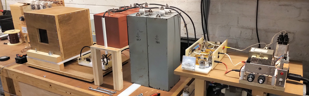
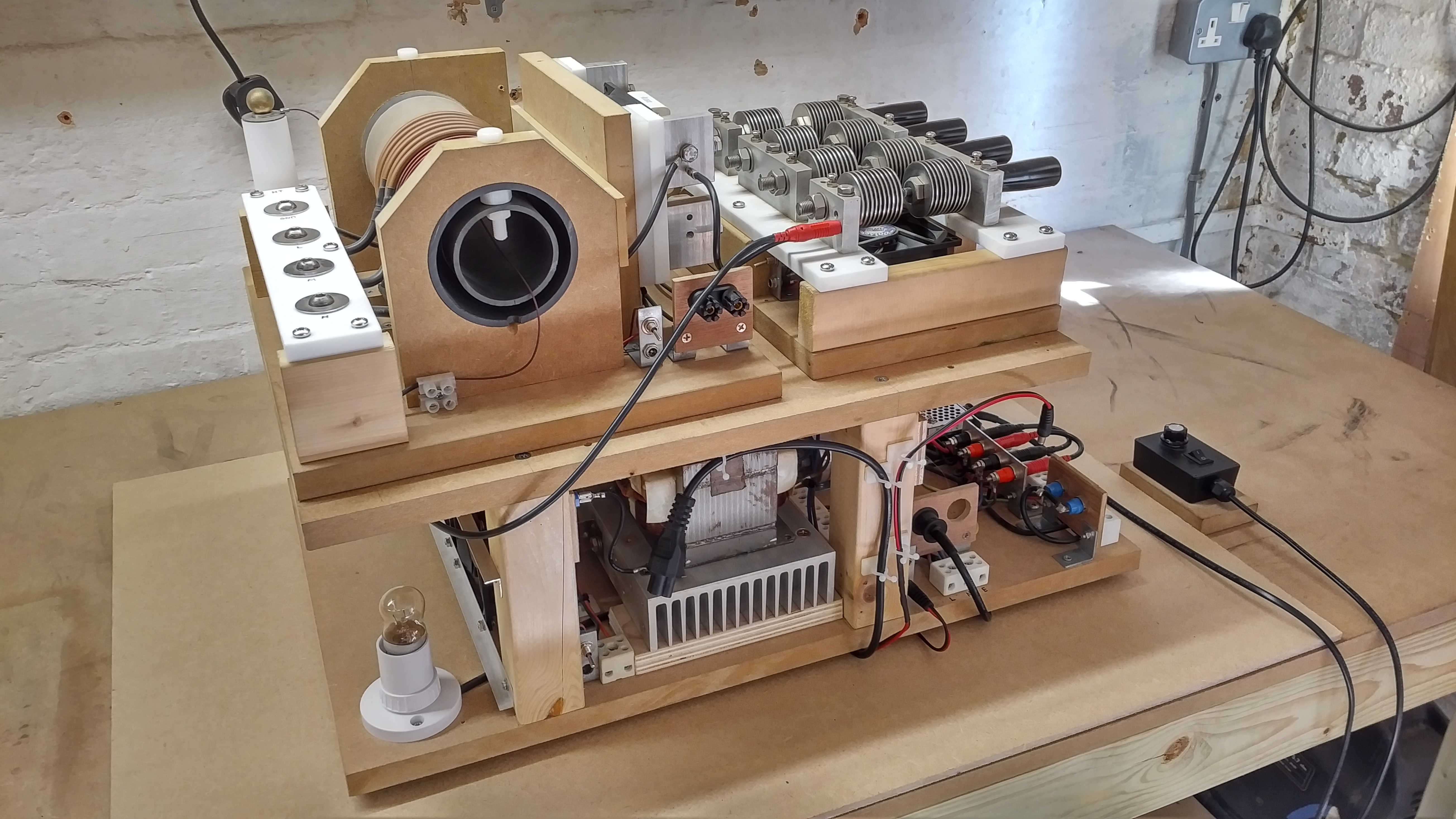
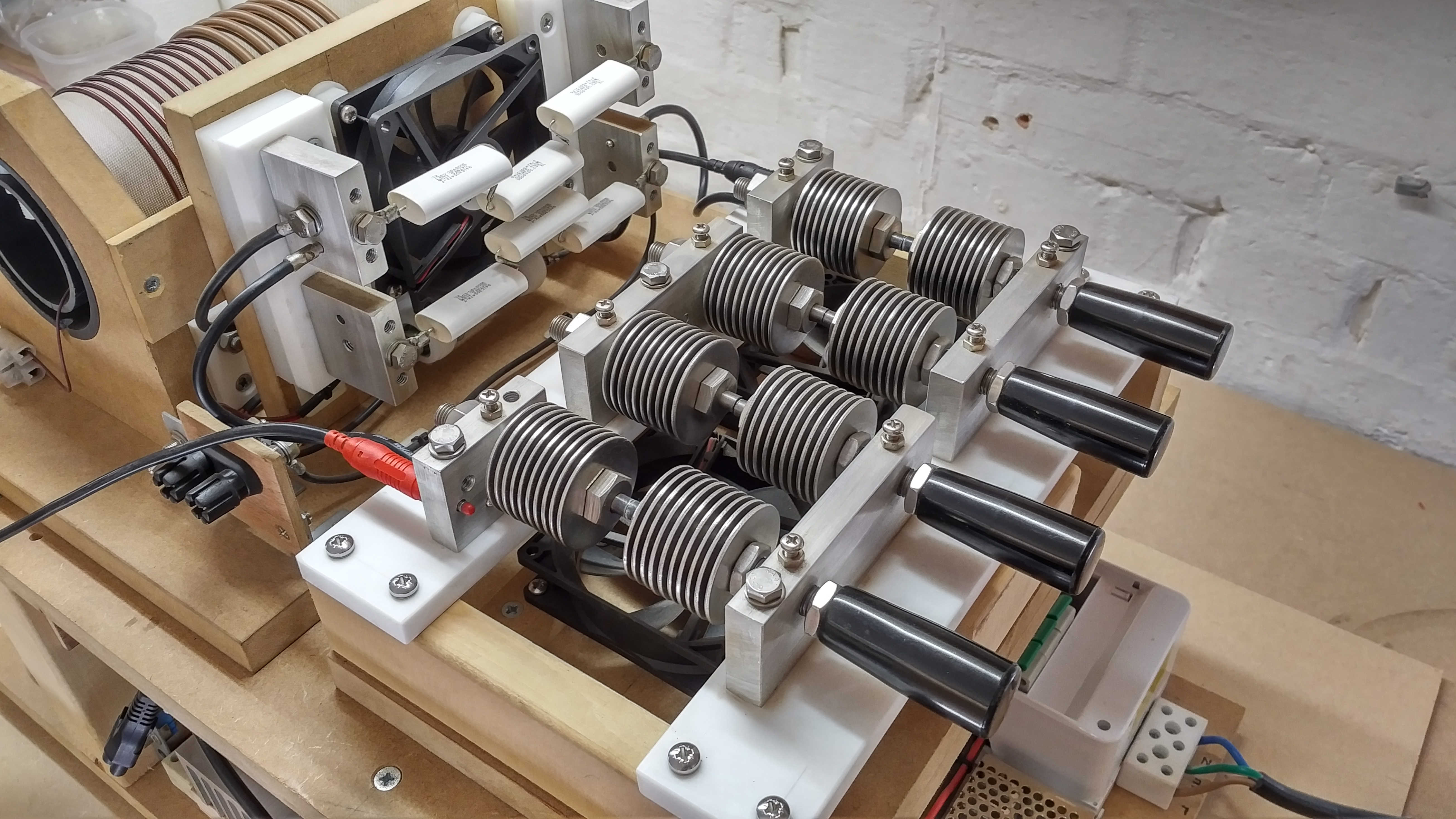
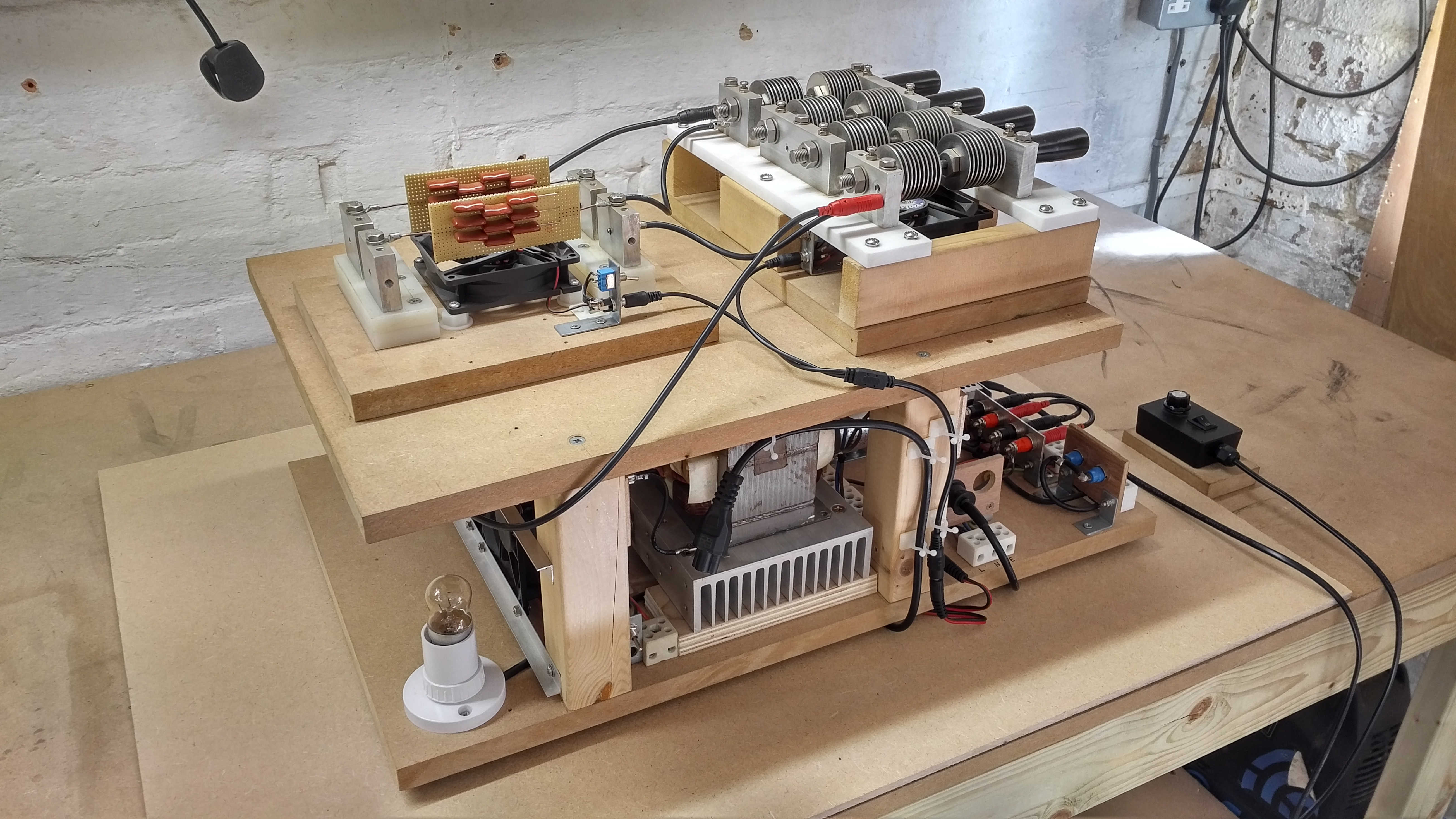
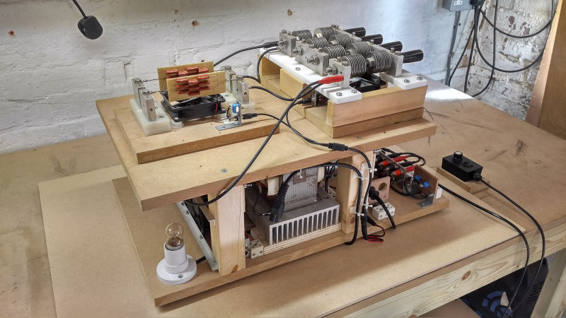
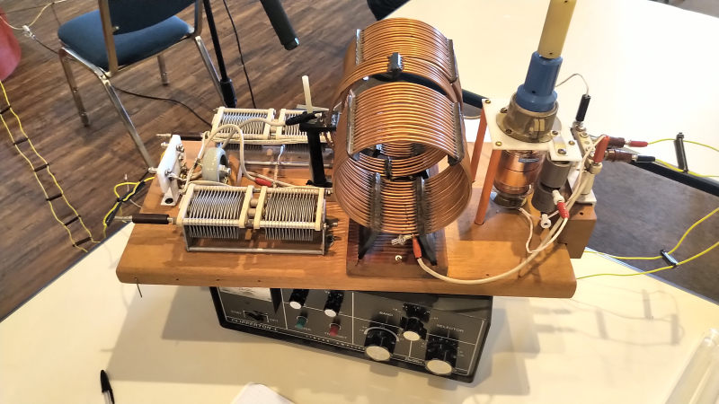
The complete spark gap generator (SGG), including the diathermy replica (DR), and the MMC capacitor bank unit, is shown in Figures 1 below, and mounted on top of, and connected to the high voltage supply:
Fig. 1.1 HV power unit connected to an H.G. Fischer diathermy replica on the top level, with the Tesla/Oudin coils on the left, and the adjustable spark gaps on the right.
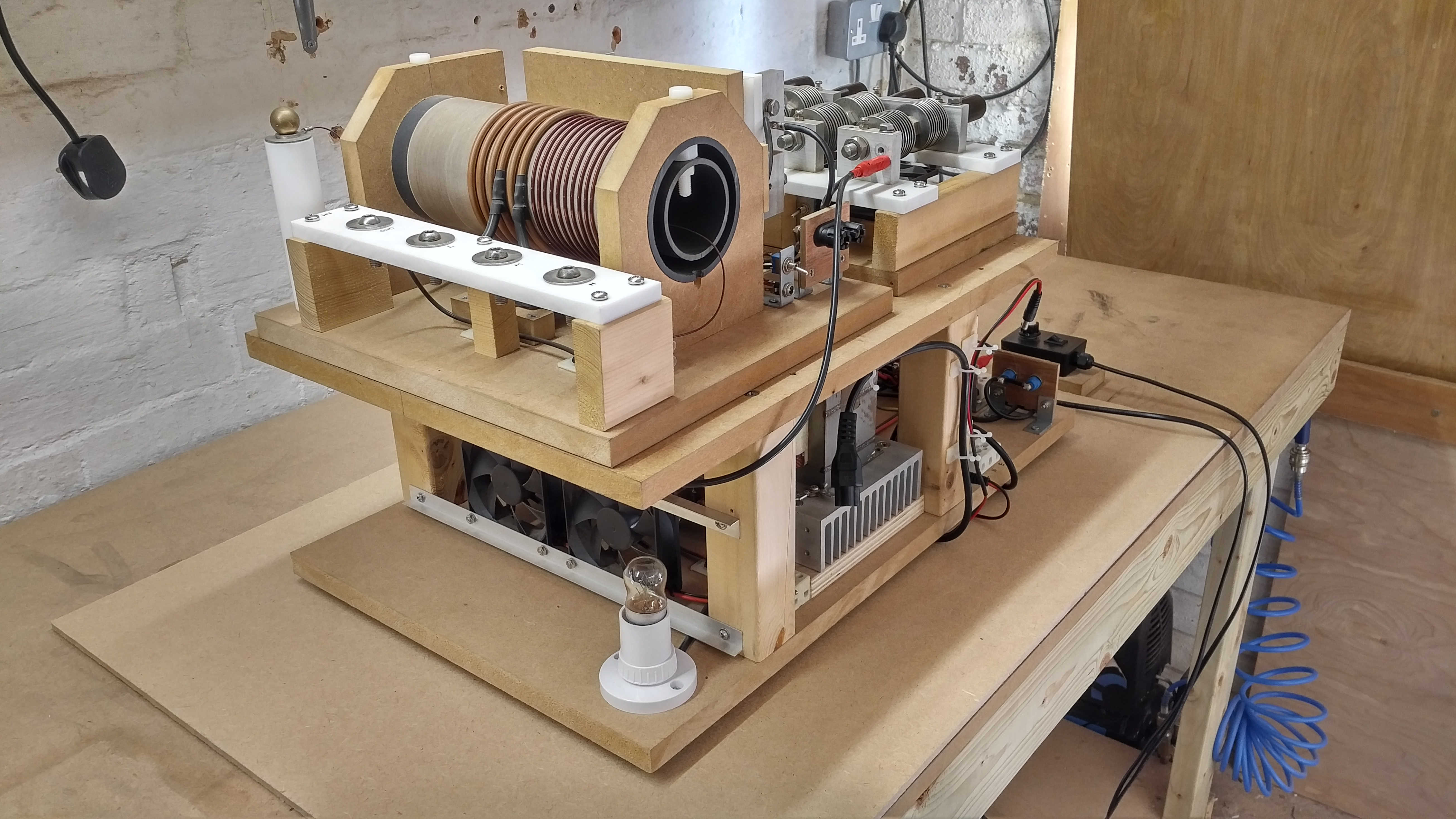
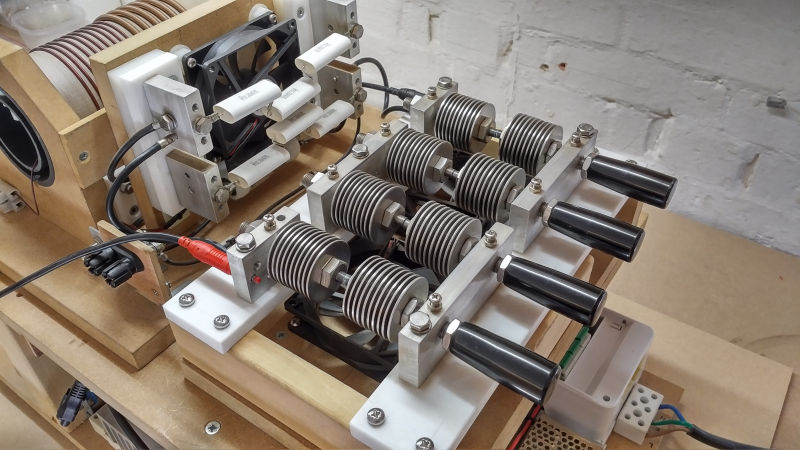
Fig. 1.2 Tesla/Oudin coil unit providing EHT output from the Tesla coil, and low, medium, and high outputs from the primary/Oudin coil arrangements. The coils are fan cooled and can run at power levels up to ~1000W continuous, and ~2000W for short bursts.
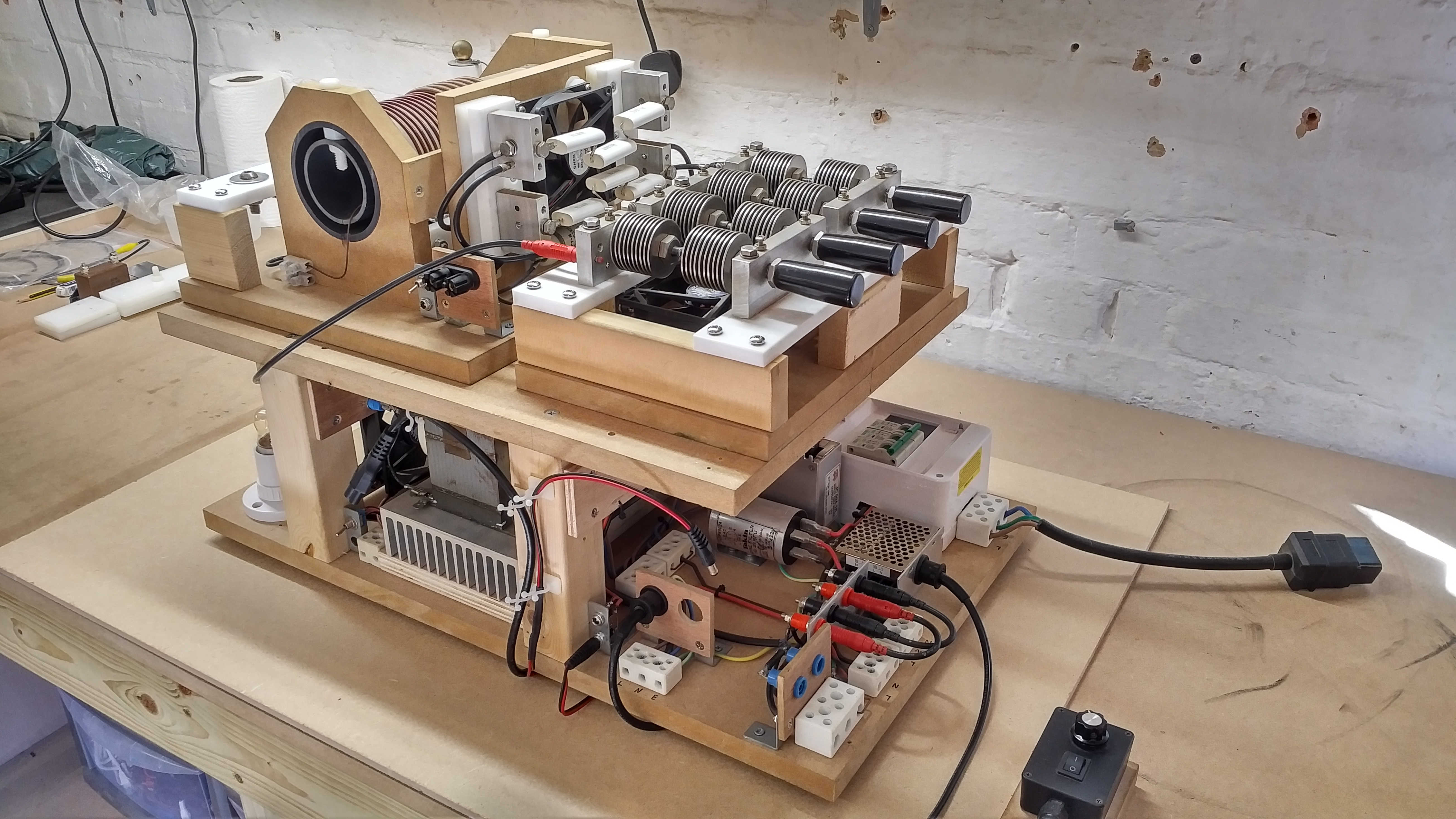
Fig. 1.3 The tungsten spark gaps can be run in series and parallel arrangements, are fan cooled, and are best driven directly in parallel from the HV unit using two MOTs in series.
Fig. 1.4 Each spark gap is a tungsten electrode pressed into a drilled, fine pitch thread, stainless steel (SS) bolt, with cooling fins made from SS washers. The final static spark unit is particularly robust and can be adjusted to operate at input powers up to ~2500W.
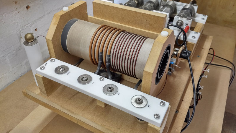
Fig. 1.5 The HV coil unit is wound according to the same parameters and dimensions as an original H.G. Fischer G2 portable unit, and displays very similar operating characteristics.
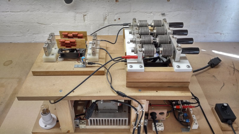
Fig. 1.6 The coil unit replaced by a cooled, direct capacitor coupled unit, designed to connect directly between the spark gaps and the flat coil tuning unit. Strong, high power, impulses can be supplied using this unit.
Fig. 1.7 The simple arrangment of the spark gaps driving fan cooled capacitor arrays makes for easy generation of high power impulses at double the line frequency 100Hz, (2 x 50Hz UK mains frequency).
Far more consideration is normally given to the experimental components (e.g. coils), their construction, dimensions, materials, and the results that they yield, and much less on the generators that produce the high voltages and currents that are used to power the experimental apparatus.
Over time this appears to have led to an “air of mystery” surrounding the generators that are used in these types of experiments, quite besides a good generator is a complex and involved process to design and build, and can take much more time than any other system component to “get right”. Certainly when I started out by watching the experimental work of Dollard et al.[1,2], I was very much left with the impression that many of the unusual results obtained were mostly a product of the special generator and components used, and the experimental coils allowed these effects to be transformed, observed, and experimented with.
I have not been alone in these impressions, as I have received very similar comments from others in the field that have not actually built a working experimental system for themselves, but rather still feel that “air of mystery” that surrounds the generator and specialised components and materials in the systems construction. Only by building or contributing to a working experimental system, (including the generator), is it possible to really dispel this “air of mystery”, as it becomes possible to understand and characterise how the generator is producing the types of voltages and currents specific to its type.
In addition to this, many of the components referred to in important works such as Dollard et al.[1,2,3], may well have been more readily available in the 80s and early 90s, but are now quite scarce, and often command high prices for working items, or “new old stock” components. For example a 1920s H.G.Fischer diathermy machine used as the primary generator in the experiments of [1] are very rare, and when they very occasionally are available, they are expensive. Without understanding what is inside a generator such as this, and how it is working, it is very difficult to know how to build a comparable generator, or whether one will be able to gain the same types of unusual electrical phenomena demonstrated in works such as [1,3].
This was certainly the place I found myself in the early days where I wanted to begin by reproducing and confirming for myself the unusual measurements and results obtained by others, before using this as an established foundation to advance further in exploring my own ideas and insights regarding electricity, and the displacement and transference of electric power. When I started out there were no good examples of a working diathermy machine currently available, (especially in the UK), so I decided to design and build a diathermy replica for myself, and using readily available materials and components. If this generator could be used to explore unusual electrical phenomena then it would certainly for me increase my understanding enormously of how such generators are designed and constructed, whilst also dispelling the “air of mystery”, and providing a generator design that could also easily be used by others in the field. Later I did finally acquire an original 1920s H.G.Fischer diathermy machine and have been able to make a characterisation and comparison between the replica and the original.
The posts reporting the Spark Gap Generator – Parts 1 and 2 are the result of building a working high power diathermy replica, which is now routinely used in my daily experiments, and has contributed significantly in bringing me to a core understanding, that all parts of the electrical system play a specific role in the generation of unusual electrical phenomena. In the exploration into the displacement and transference of electric power each part of the system apparatus must first be measured and characterised carefully to establish a well tuned and balanced overall system, and where the electric and magnetic fields of induction are balanced and in a state of dynamic equilibrium.
From this point it is possible to experiment directly into the properties of electricity, and come to an understanding that the unusual phenomena observed are a product of the inner workings of electricity itself, where the generator and experimental apparatus are necessary to set up the conditions and boundaries required to explore these inner properties. The properties of electricity are there to be revealed rather than “generated”, which also assists greatly in dispelling the “air of mystery” that the generator is the source of the unusual phenomena, but rather, the instrument that provides the necessary tension to trigger the imbalance of the electric and magnetic fields of induction, and hence to observe electrical phenomena within the system. The differences here are subtle but hugely important to the overall understanding of electricity and particularly displacement of electric power.
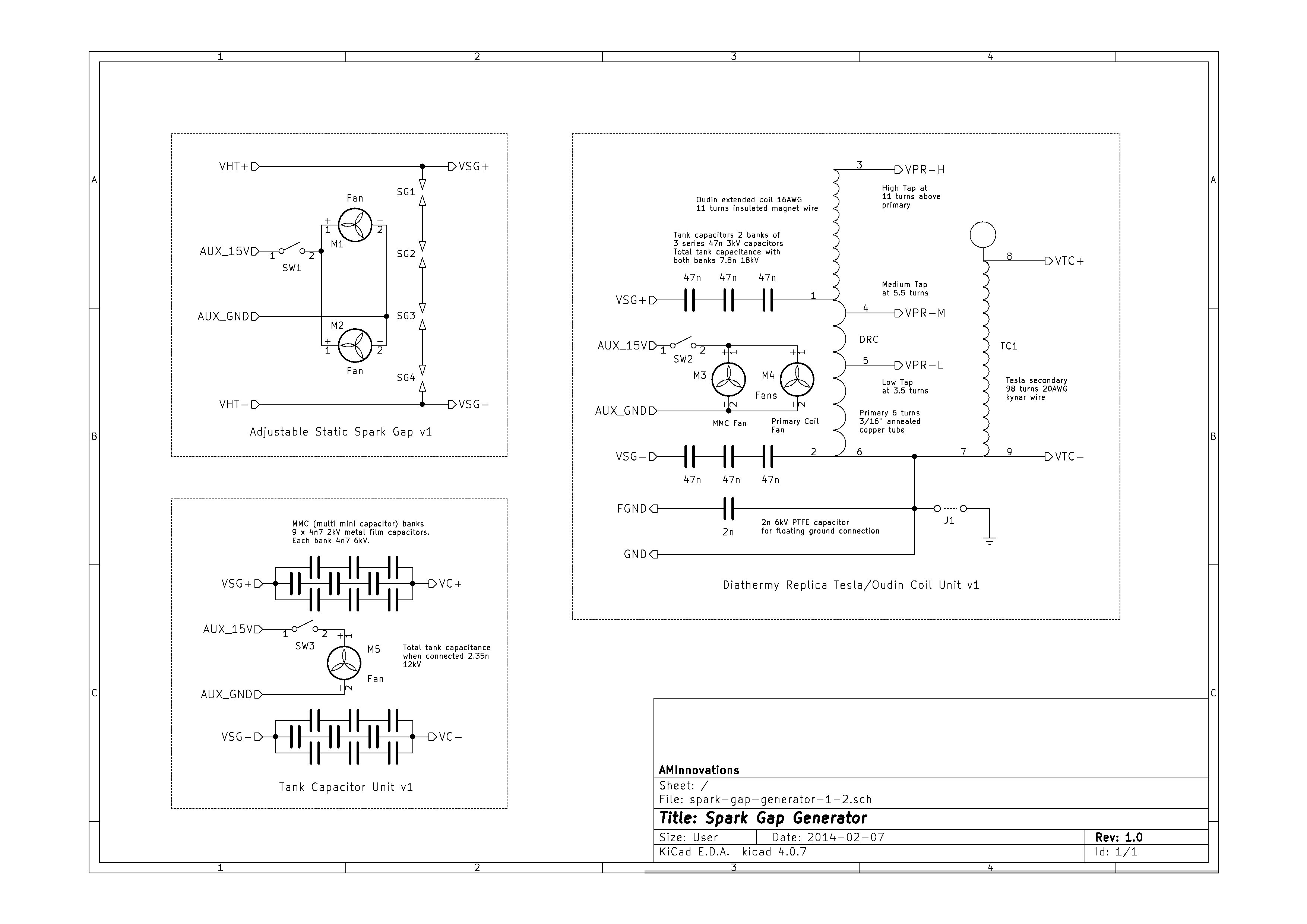
The circuit diagram for the SGG and peripherals is shown in Figure 2 below, or click here to view the high-resolution version.
Fig. 2.1 Spark gap generator schematic showing the static spark gap, the diathermy replica unit, and the tank capacitor unit.
In the early days in order to replicate the experiments and results of Dollard et al.[1] , it was considered that the diathermy replica (DR) should be as close as possible to the original, which of course posed a challenge when there was no original from which to take measurements, dimensions, construction methods etc. To overcome this a range of references from the internet were studied, along with available circuit diagrams. The most useful references proved to be a combination of material from [3,4,5], and allowed key dimensions and some circuit component values to be extracted from the images and videos.
Click on the following links to view circuit diagrams for various original H.G. Fischer (HGF) diathermy machines, the Model G2, the Model H, the Model CDC, and the Model A[4].
In any Tesla or resonant coil design it is first necessary to define the desired properties of the secondary coil. With this defined the primary and other components of the system can be designed around the secondary properties. In the case of the DR, and in the absence of any good measurement data, e.g. the resonant frequency of the HGF secondary, the DR secondary was designed according to the known and available dimensions of the HGF secondary, the wire size and type, and the number of turns, (mostly gained from [5]). The dimensions and wire were then adjusted for readily available materials and then key parameters extracted using the software Tccad 2.0[6]. The DR secondary coil properties were adjusted primarily to match F0 the primary resonant frequency of the secondary coil, while keeping the physical dimensions as close as possible, whilst using readily available material types and sizes. The original HGF and the designed and adjusted DR properties are shown in the following table:
Original H.G. Fischer Model G Diathermy:
From reference pictures and video[5]:
Turns: 90
Wire: Solid copper 20 AWG cotton-clad, total diameter 1.0mm
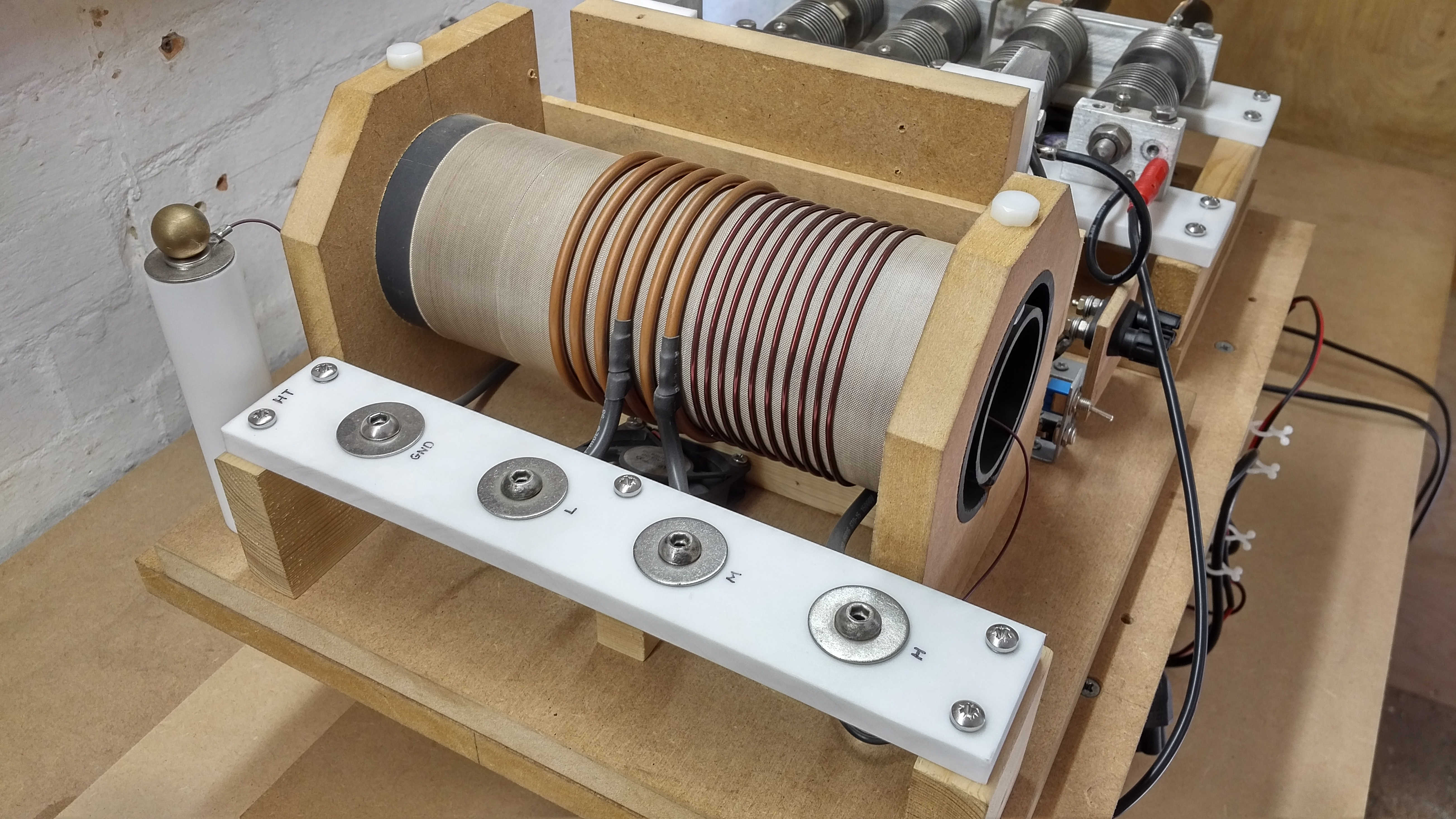
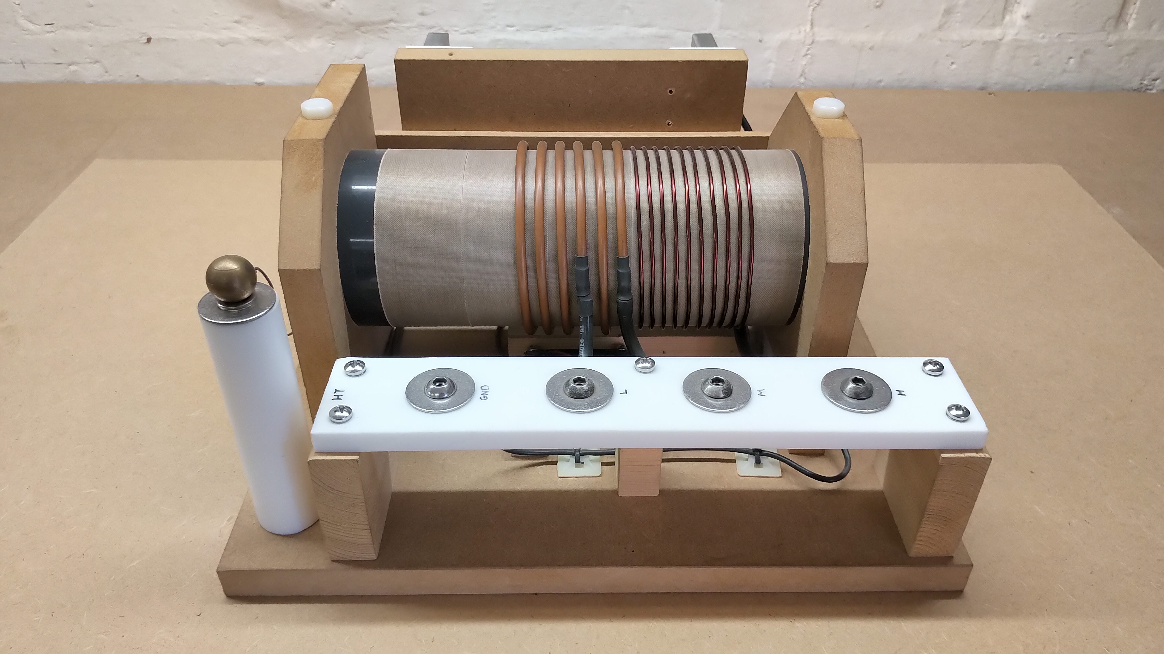
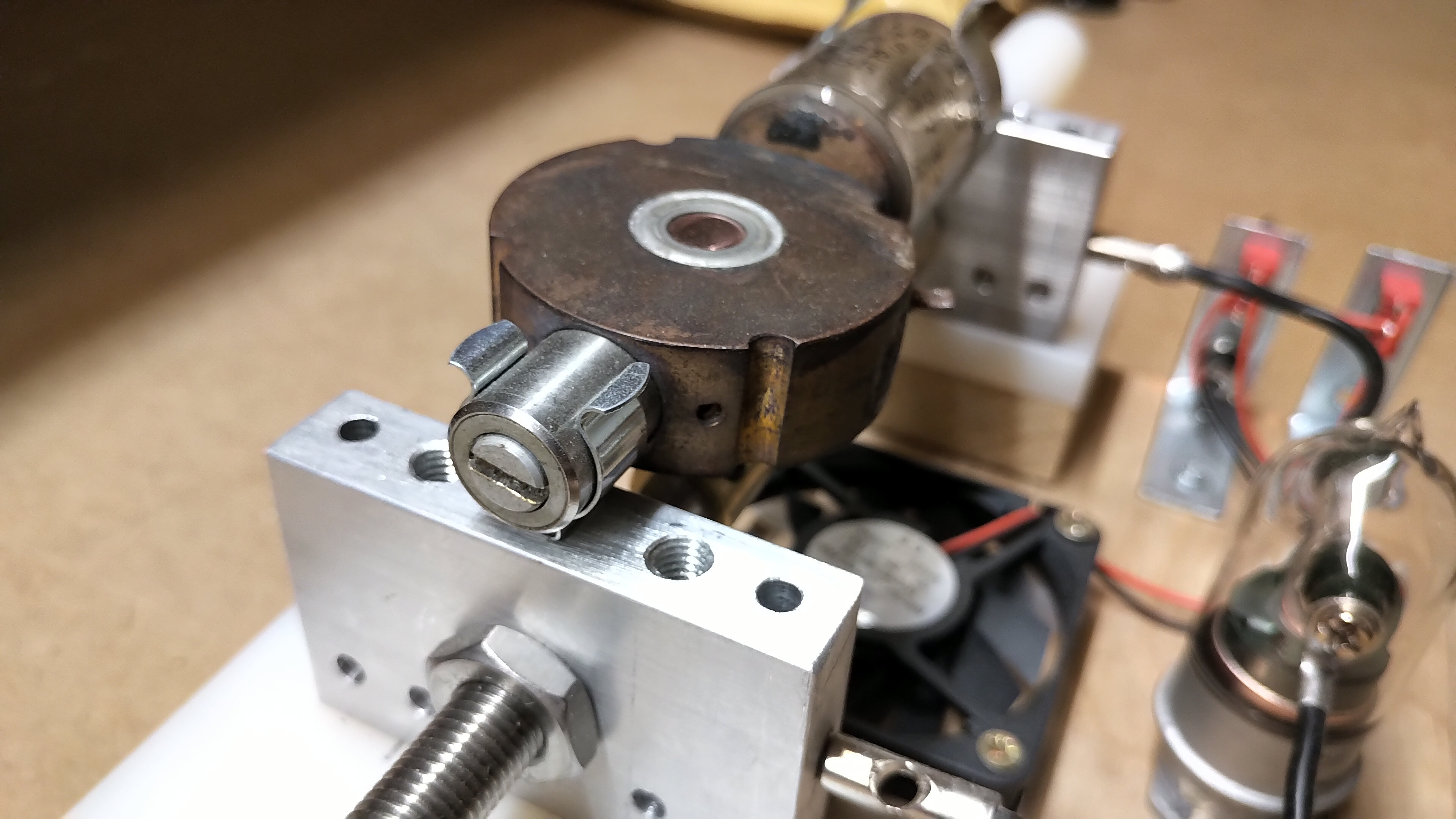
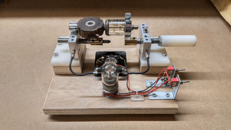
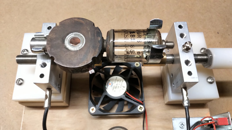
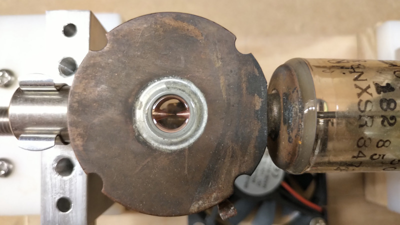
Figures 3 below show how the Tesla/Oudin unit was constructed, and the types of materials used in a simple open structure that can be easily adjusted and modified according to the experimental requirements. Components are mounted on a mdf wooden base, and conductors insulated from the mdf using PTFE and Nylon 66 mounts, bolts, and nuts.
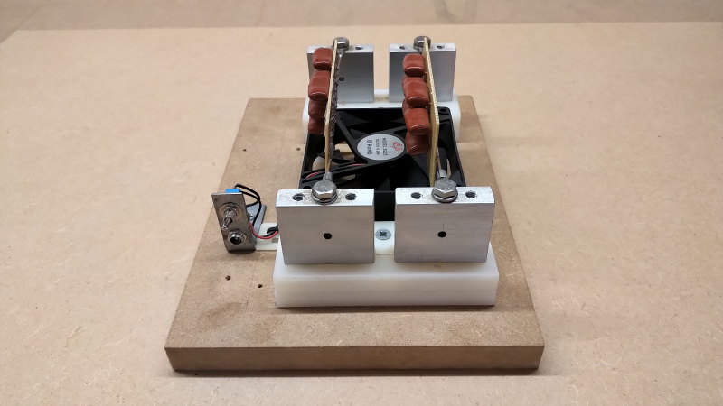
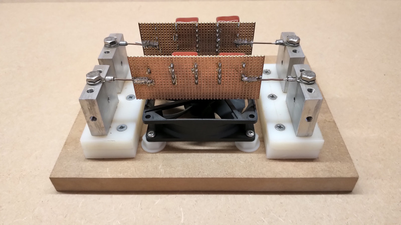
Fig. 3.1 The DR module showing the copper primary coil with extension coil, the output taps to the low, medium, and high outputs, and the secondary coil output connected to a brass ball.
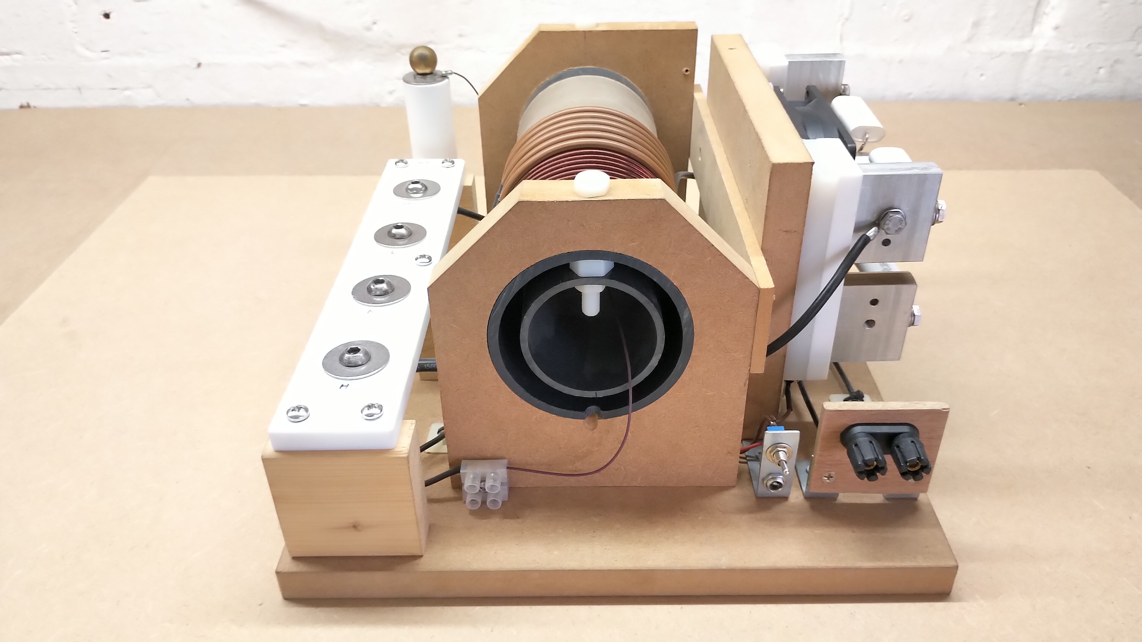
Fig. 3.2 The secondary coil is attached inside the primary plastic tube using nylon locating bolts and a nylon nut as a spacer.
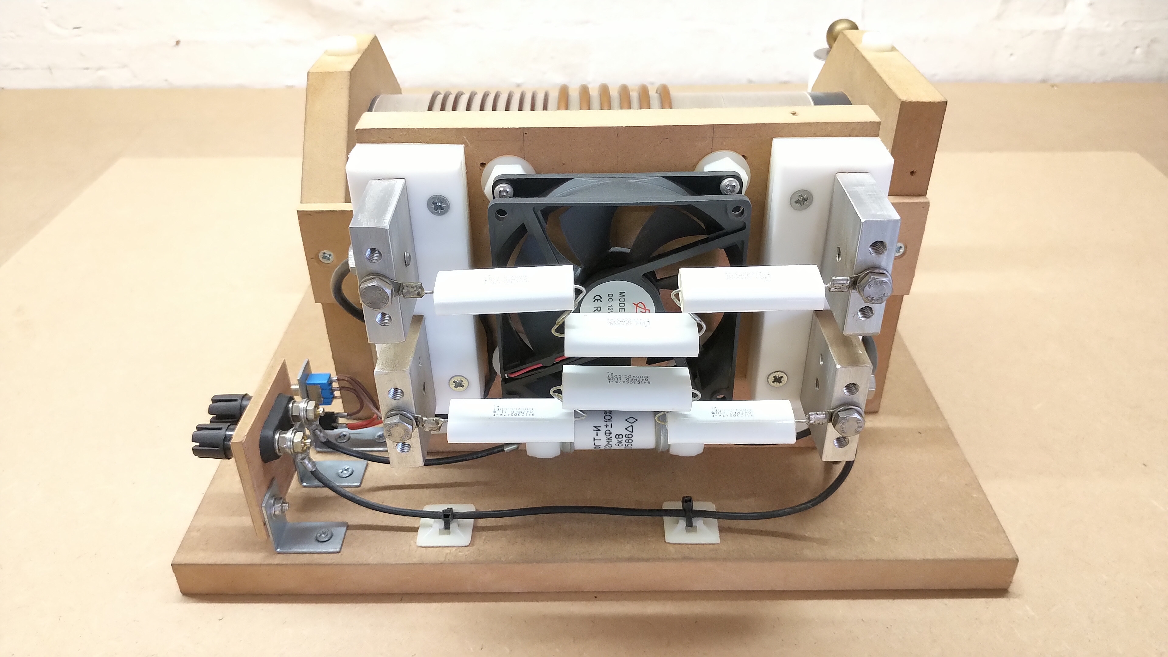
Fig. 3.3 The primary tank capacitors are two series strings of Cornell Dubiller 3kV 47n high voltage capacitors, which are force air cooled when running at high output powers.
Fig. 3.4 The secondary coil is wound using PTFE coated 22AWG silver coated (Kynar) wire, and the output fed to a brass ball mounted on a PTFE insulated mount.
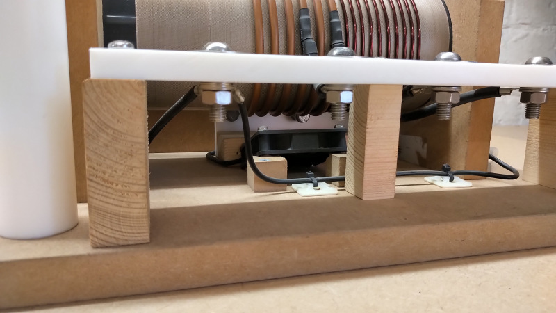
Fig. 3.5 The tank capacitors are mounted on aluminiium supports which in turn are insulated from the wooden base using PTFE/Nylon mounts.
Fig. 3.6 The secondary coil is suspended inside the primary by nylon bolts, and can easily be removed and replaced with different secondary coil's of different specifications.
Fig. 3.7 The secondary coil is wound on a polypropylene pipe coated with PTFE tape to improve the thermal barrier between the pipe and the wire when operating at high output powers.
Fig. 3.8 The primary coil is cooled using a fan mounted beneath the coil, and allows output powers in excess of 1.5kW to be sustained without over-heating the module.
The formers of the primary and secondary coils were first coated with PTFE tape to improve the thermal barrier between the coil and the polypropylene former material when running at high output powers. In addition a small low voltage fan was located under the primary coil to help keep the primary cool at sustained high power outputs. The Tesla EHT output and the HT output taps are all mounted on PTFE insulators both for electrical isolation, but also for good resistance to melting and burning which can occur when drawing discharges from these terminals. Nylon 66 can also be used here, but has lower thermal resistance to discharges, but has the benefit of being a much cheaper material than PTFE.
It is important to note that the secondary coil is located in the primary at the opposite end to the Oudin extended coil. In an early version of the DR the secondary was incorrectly located at the same end as the Oudin extension, which because of the increased tension in both coils easily causes breakdown between the two coils, and led to burn-out of the first secondary coil. The tank capacitor banks are made from 3 series connected Cornell Dubiler 941C03 series 3kV polypropylene film capacitors each of value 47nF, which combined gives 15.7n 9kV for each bank. These tank capacitors have been proven to be long-lasting, and robust, and have never been changed, even with input powers in excess of 1.5kW and even up to 2.2kW for short bursts of power.
The tank capacitors are force air-cooled, and mounted on insulated conductors which allow for easy connection and adaption to the circuit under test. The capacitance of the tank was initially higher at around 47n to match more closely the HGF schematic of the Model A, but was reduced to its current value after the real HGF was acquired and measured. At 47n the available output power was quite a bit less than with 15.7n per tank, as the primary resonance is pushed lower and further away from that of the secondary, hence reducing the primary currents, and hence the power coupled from the primary to the secondary.
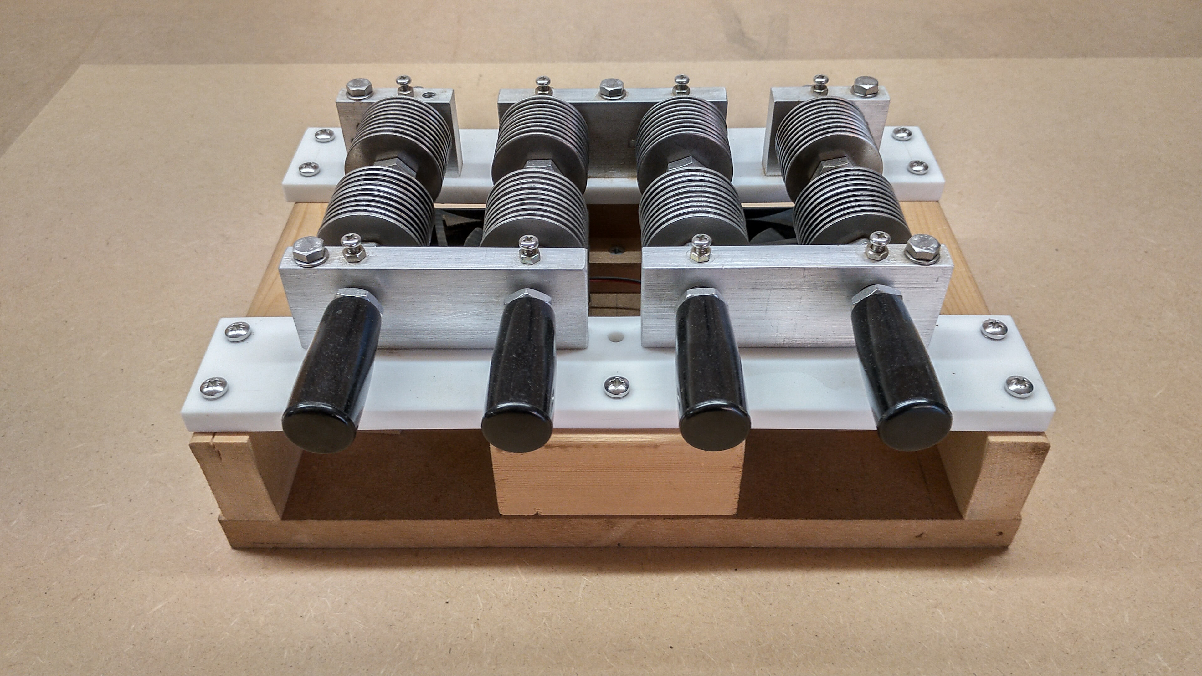
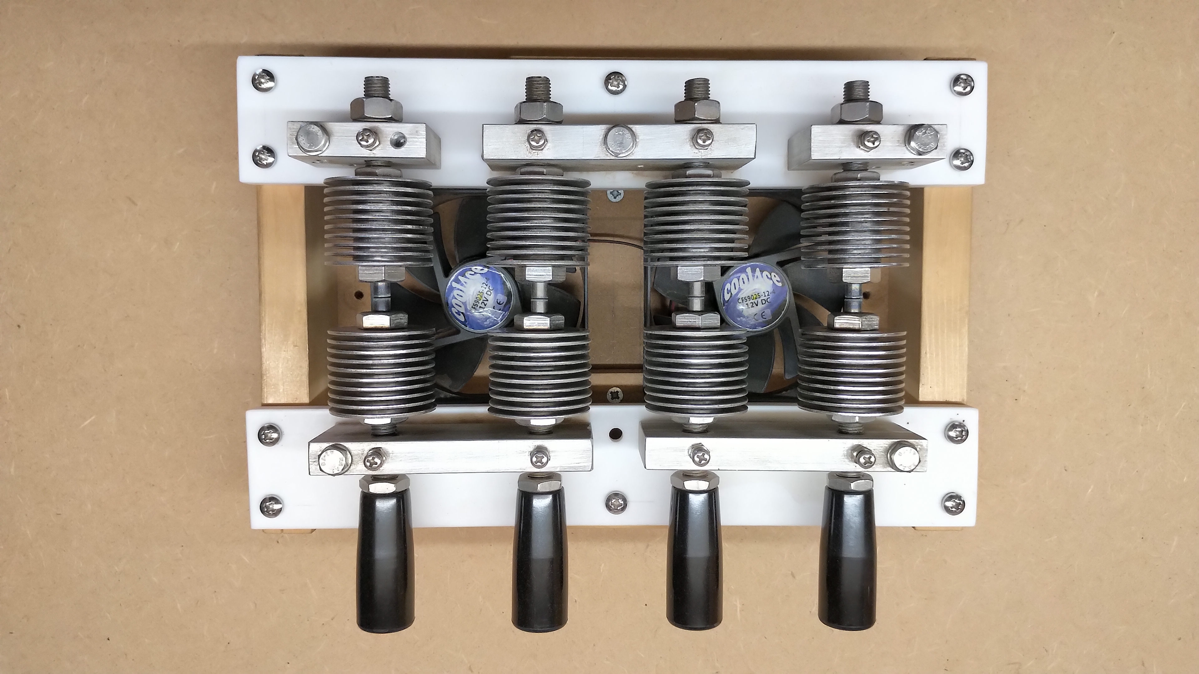
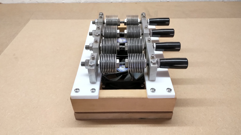
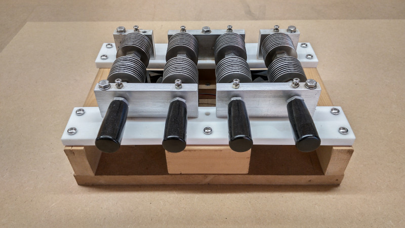
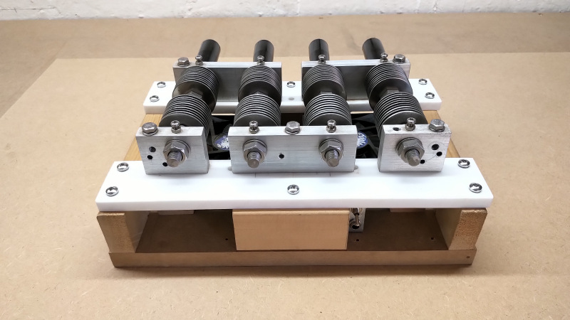
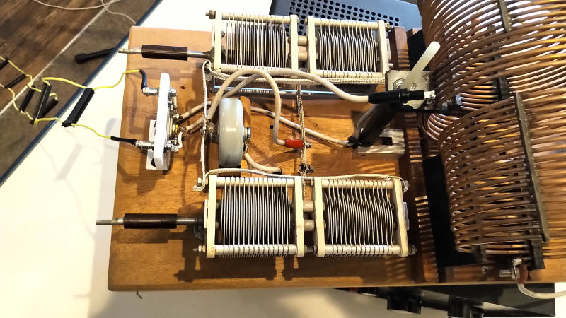
Figures 4 below show how the static spark gap (SSG) unit was constructed.
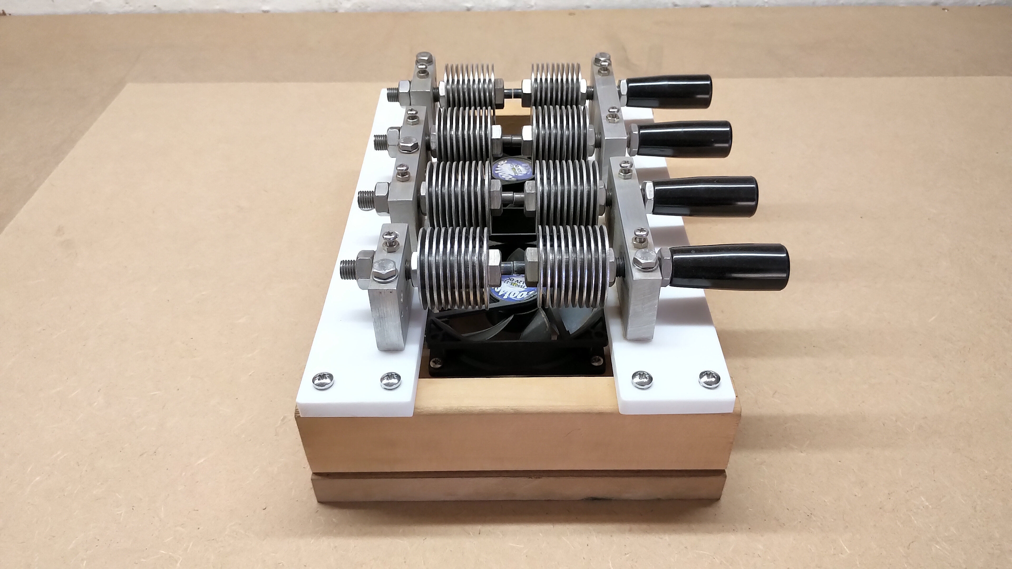
Fig. 4.1 The SSG module showing four static spark gaps connected in series via their aluminium mountings.
Fig. 4.2 The spark gap spacing for each gap can be fine adjusted using the insulated handles, and can be tuned for optimum performance whilst running.
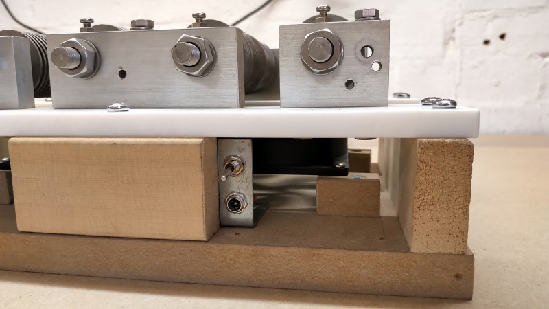
Fig. 4.3 The aluminium mounts are insulated from the wooden base by PTFE blocks. The thread of each spark gap bolt is tensioned by a small nylon insert which is compressed using an M4 machine screw and locking nut.
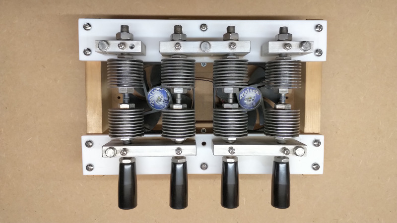
Fig. 4.4 The four spark gaps are force cooled by two fans positioned directly under the gaps. Force cooling allows the gaps to be run in excess of 1.5kW for sustained experimental periods.
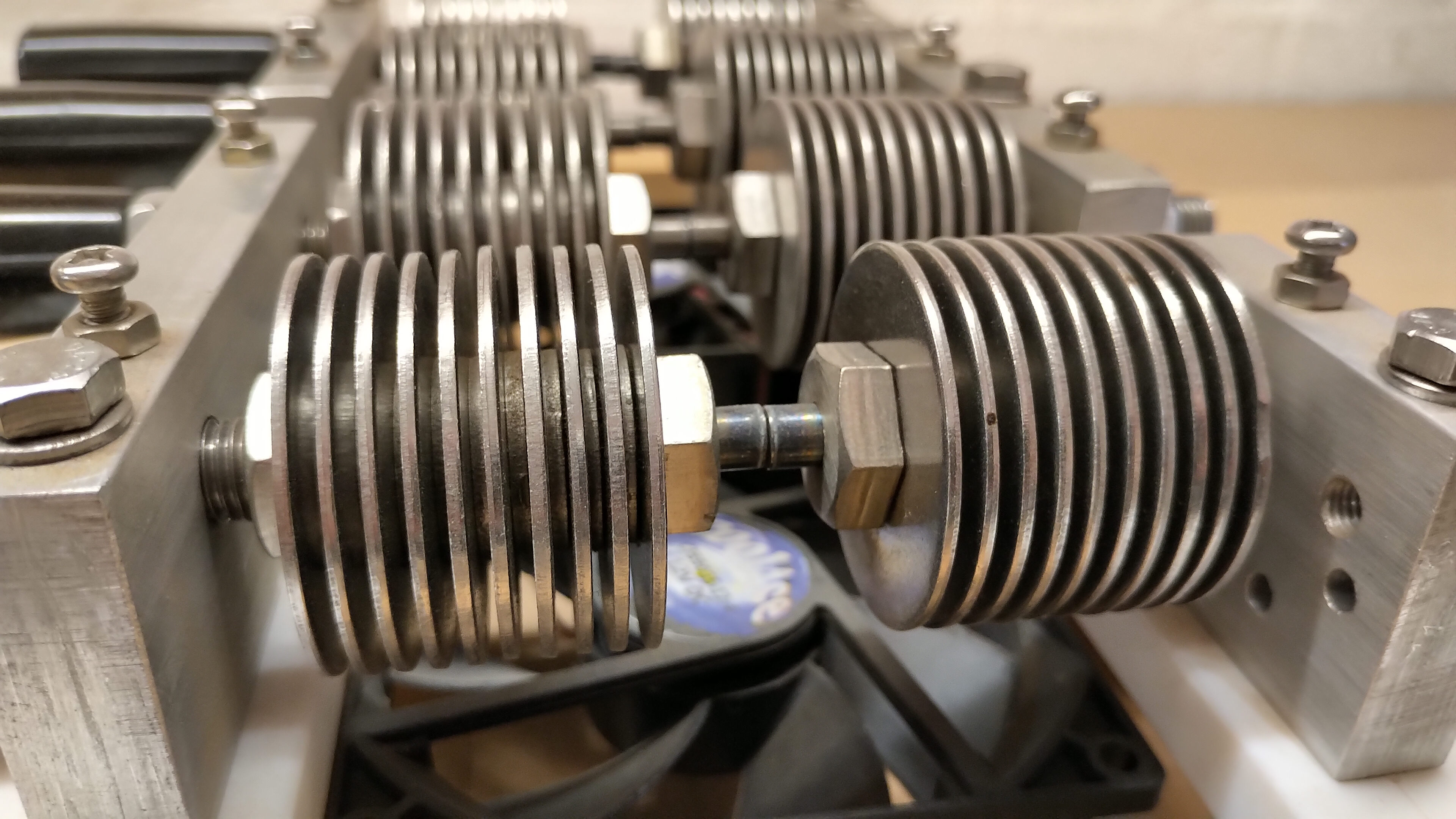
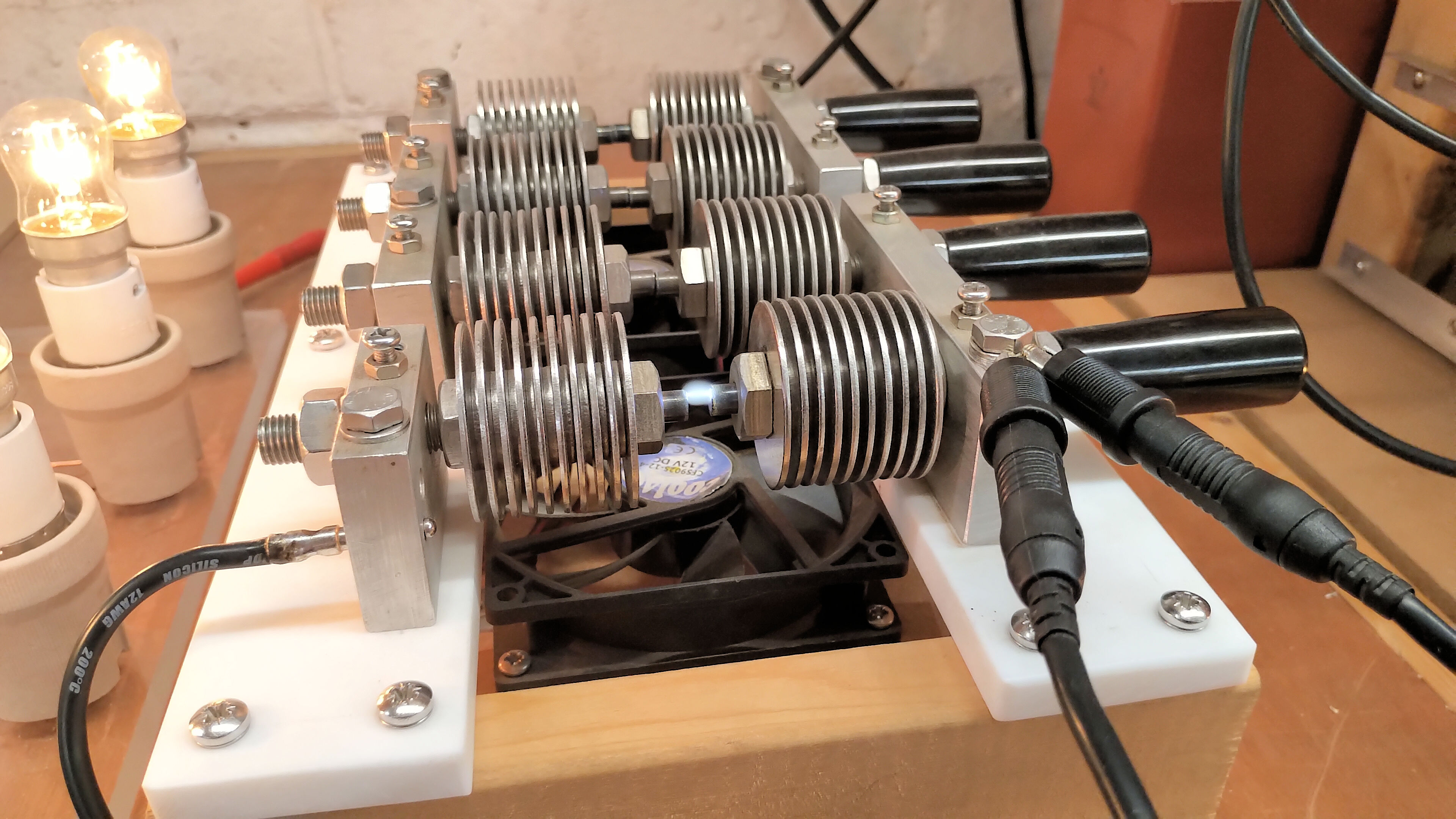
Fig. 4.5 Each gap is made from a tungsten rod pressed into a stainless steel bolt with alternating size stainless washers acting as cooling fins.
Fig. 4.6 The fans are powered by a switched low voltage supply isolated below the high voltage gaps by the PTFE mounts.
The SSG unit was at the time the most difficult unit to build when only a large pillar drill, large vice, and bench sander were available in the workshop for mechanical construction. Each electrode of the spark gap is made from 1/4” diameter 99.9% pure tungsten rod 1″ long, (not to be confused with tungsten carbide rods), which were pressed using the vice, into the centre of a drilled A2 stainless steel fine pitch bolt. The bolt had a 6.2mm hole centre drilled, by mounting the bolt in the drill chuck and clamping the drill stationary on the stage, and opposite to how a drill press is normally used. This arrangement made a very rudimentary “lathe” and made it easier to drill a centralised 1.5″ hole down the centre of the bolt. The tungsten electrode was then pressed into the bolt leaving 5mm externally for the spark electrode. Alternating stainless steel washers (large and small) were then threaded onto the bolt and finally tightened with a thin stainless steel nut to form the cooling fins of the electrode body.
Each pair of electrodes were then mounted in threaded aluminium blocks, locked in place with a nut on one side, and with a threaded bakelite handle on the other, to allow adjustment of the spark gap space by winding the bolt in or out of the aluminium block. The aluminium blocks were arranged and mounted to form a series connection of all four spark gaps, and also allowing for tapping from any of the 4 stages for experiments using a single gap, all the way up to 4 series gaps, or 4 parallel gaps with shorting shunts. The adjustable electrode was tensioned in the alumium thread by a small compressed nylon rod, ( from an M3 nylon bolt), which was inserted in a vertical hole drilled above the thread, and then tensioned using a screw locked in the correct place by a nut.
The aluminium spark gap blocks are mounted onto PTFE insulators and then mounted to a wooden base where each gap is suspended above force cooling provided by a pair of low voltage plastic fans mounted into the base of the unit. Overall the SSG unit is robustly constructed and can withstand very large powers in constant use. Tuning of the gaps for optimal running can be made carefully during operation via the four insulated adjustment handles, and is demonstrated in the operation video in Part 2.
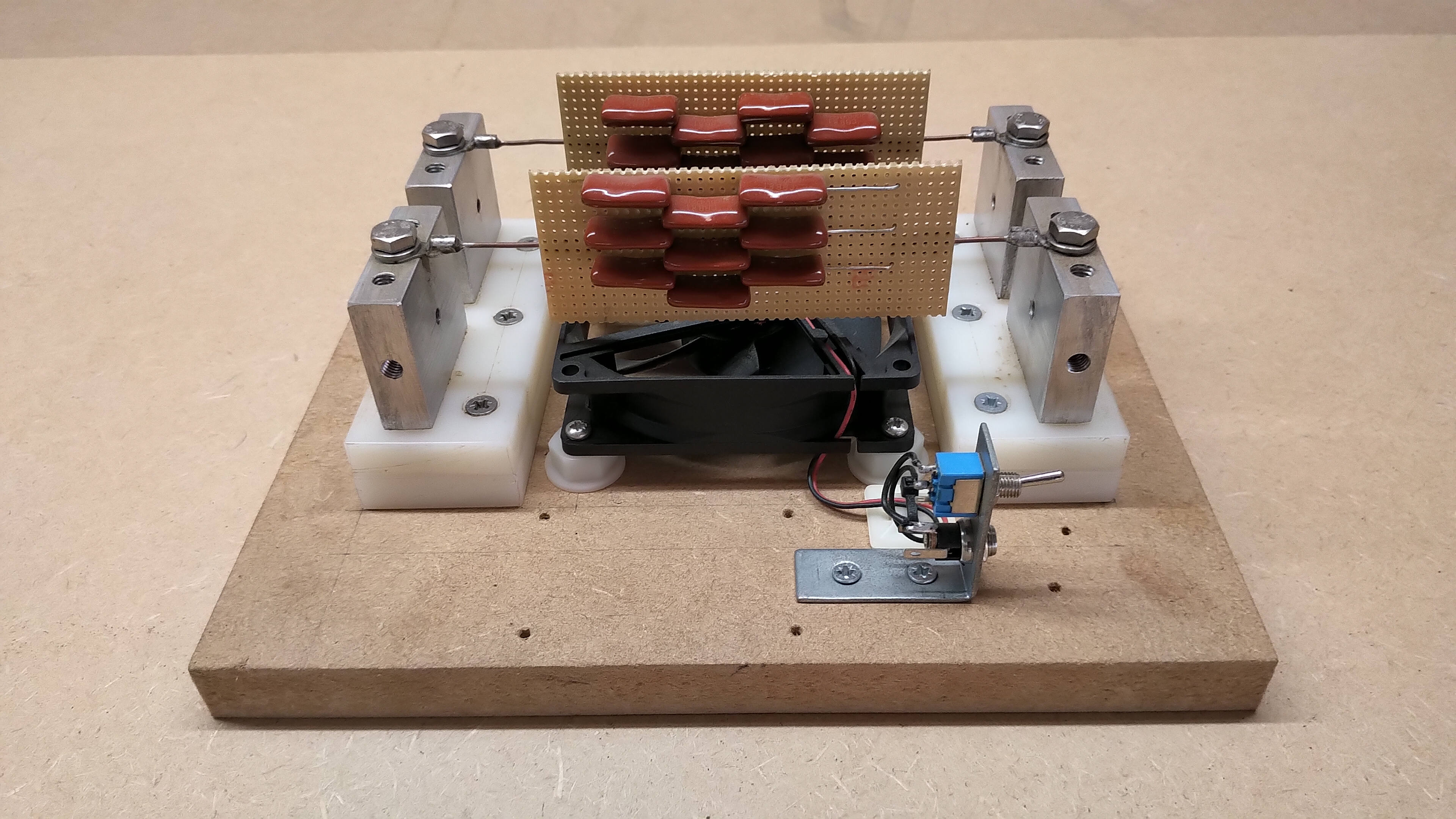
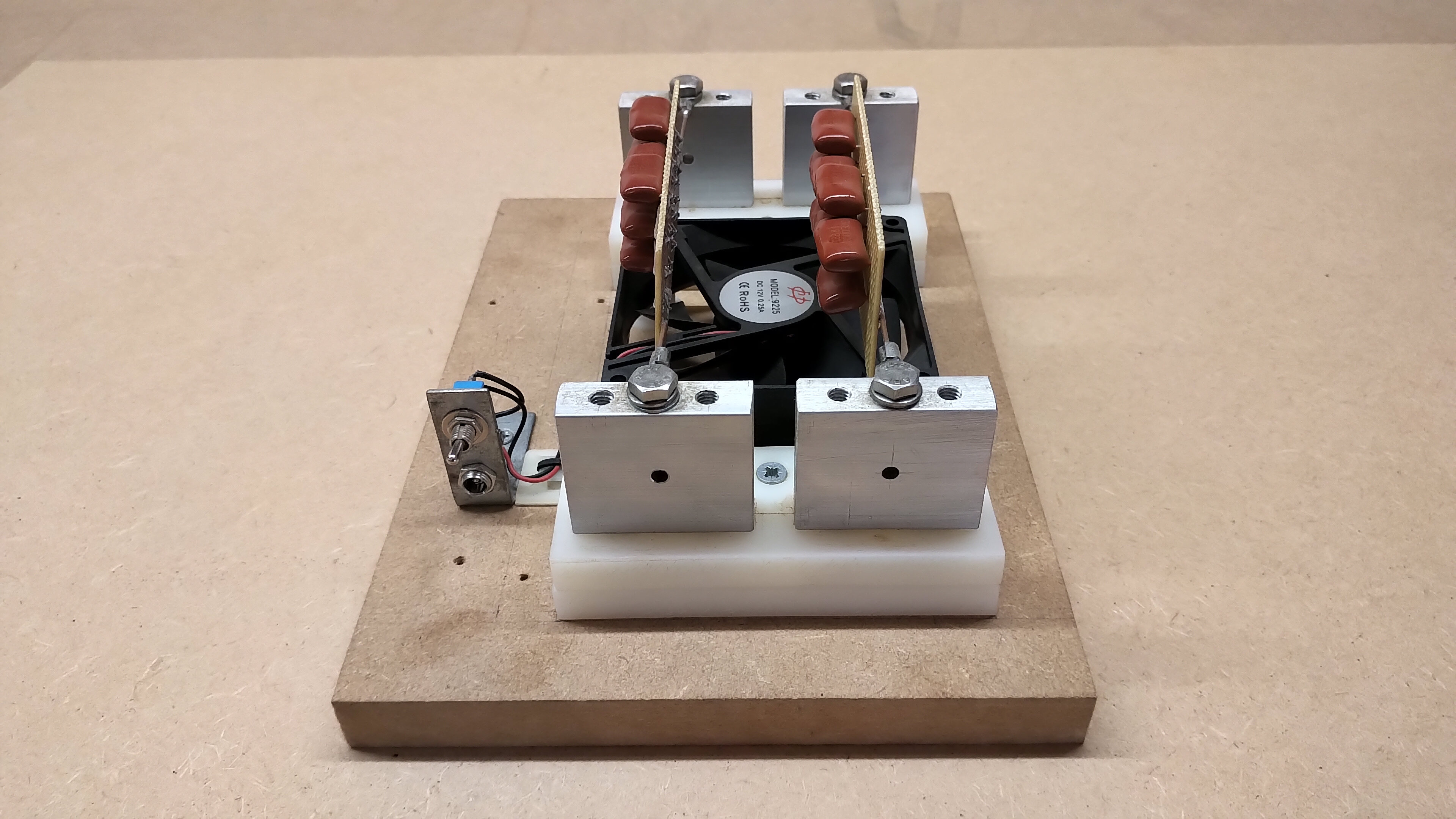
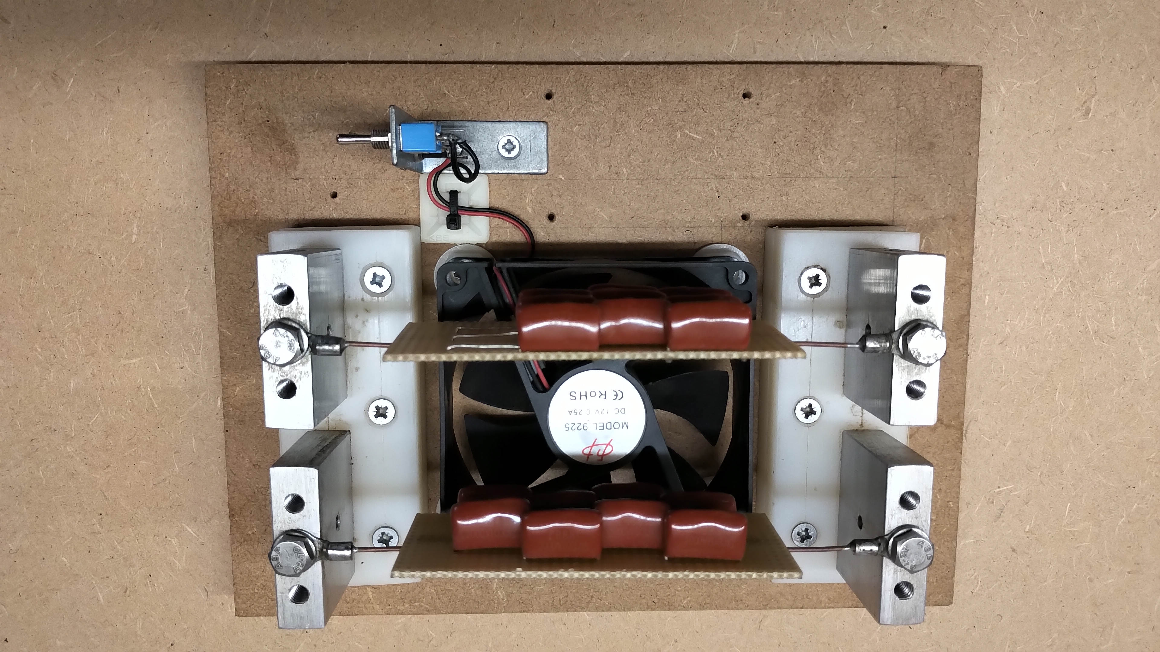
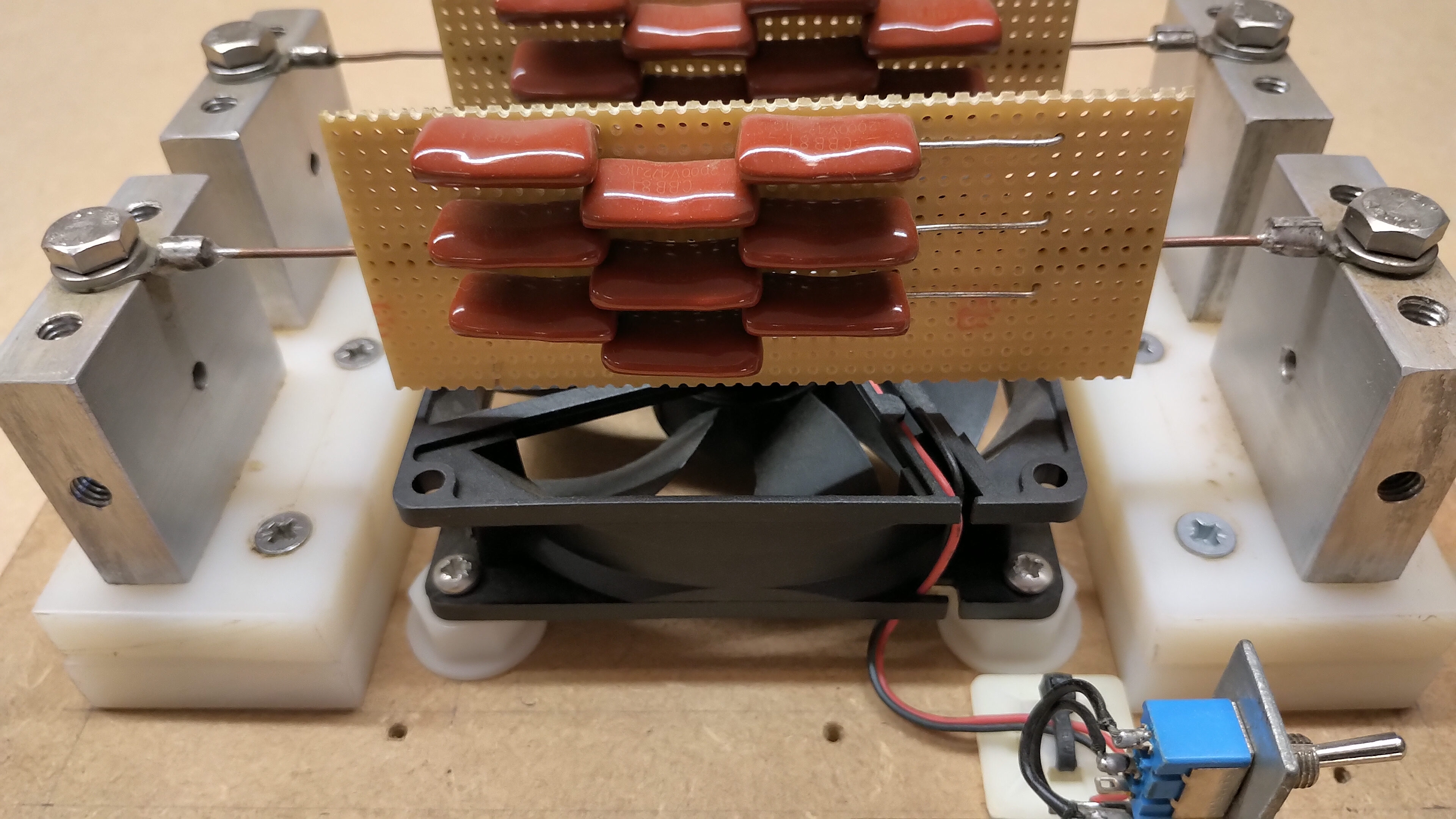
Figures 5 below show the MMC tank capacitor bank (TCB) which was used to remove one of the tuned primary stages, and hence increase the efficiency and optimisation of the generator driving, for example, the tuned primary of a TMT (Tesla magnifying transformer).
Fig. 5.1 The tank capacitor unit showing the MMC capacitor banks, each a 4.7n 6000V metal film capacitor.
Fig. 5.2 Insulated aluminium blocks mount the MMC banks over forced air cooling powered by a switched low voltage fan.
Fig. 5.3 With forced air cooling the MMC banks work sustainably up to 500W input power. Larger MMC banks can be used for higher input powers.
Fig. 5.4 The MMC banks are mounted on veroboard, and are arranged in three parallel strings to increase current handling.
Fig. 5.5 The MMC banks are arranged in strings of three series capacitors which gives a total maximum voltage handling of 6kV.
The SGG used with the DR as a generator is most commonly connected with one of the L, M, or H outputs to the primary stage of a tuned TMT, of which the primary stage would typically consist of a coil with a parallel tuning capacitor. In this arrangement the DR, which in itself is already a tuned primary stage, is now connected to another tuned primary stage. Whilst this was useful for preliminary experiments in confirming the key experiments and results of Dollard et al.[1,2] and keeping the generator as close as possible to an original HGF, it has been shown to be more efficient to eliminate the double tuned primary stage by removing the DR and placing the TCB in its place.
The TCB is simply a standalone capacitor unit exactly the same design as used in the input to the DR. Here the TCB is shown with two pcb MMC banks, but the Cornell Dubilier 941C03 series banks could equally as well be mounted in the same way. Figures 1.6 and 1.7 show how the TCB is connected directly to the SSG, and then in turn the output of the TCB is connected directly to the input of, for example, the tuned primary of a TMT, or some other experiment or load. This creates a resonant drive circuit with the TMT coil in series resonance with the TCB capacitors, and is exactly the same arrangement as internally for the DR, and the HGF. Use of the TCB in replacement for the DR has allowed for an easier and more accurate resonant match between the SSG unit and the TMT load, and with greater power transfer between the two units. Impedance measurements are also simplified by removing one resonant circuit from the generator chain. A very wide range of capacitors can be mounted on the TCB, and for higher power experiments up to 2.5kW output power, force cooling is available via the low voltage fan in the base of the unit.
Overall the spark gap generator whether used with the DR unit or the TCB unit at the output, has proven to be a robust and reliable generator for a wide range of experiments. It has enabled the replication of the key experiments as presented by Dollard et al.[1,2,3,4], as well as forming a flexible and powerful tuned static spark generator for my own experiments in the displacement and transference of electric power, as well as telluric transmission experiments.
Click here to continue to part 2 of the spark gap generator where the operating characteristics are measured both in frequency and time, as well as a short video to show its general operation and running.
1. Dollard, E. & Lindemann, P. & Brown, T., Tesla’s Longitudinal Electricity, Borderland Sciences Video, 1988.
2. Dollard, E. & Brown, T., Transverse and Longitudinal Electric Waves, Borderland Sciences Video, 1988.
3. Dollard, E. & Mackay, M., Tesla Radiant Energy Experiment, Bedini-Lindemann Conference, June 29-30, 2013.
4. Mackay, M. & Dollard, E., Tesla’s Radiant Matter Replication, 2013, Gestalt Reality
5. Sergey Z., Fischer Diathermy Narrating and Exploring a 1920’s Tesla Coil, May 2014, Youtube
Part 1 of the spark gap generator covered the major components of the system, along with the design steps taken to build a diathermy replica unit (DR). In this part measurements are carried out both in the frequency and time domains, to further understand the operating characteristics, and how best to match the output of the generator to the experimental load. In this part there is also consideration as to how the generator transforms the incoming mains supply to an output suitable for experiments in the displacement and transference of electric power.
The primary purpose of any generator within such an experimental system, arranged to investigate the inner properties and workings of electricity, is to provide the necessary tension to the experiment, in order to change the balance of the electric and magnetic fields of induction within the local region of the experimental system. It is considered that changing the local balance of these fields in turn couples to deeper properties within the energetic dynamics and wheel-work of nature, which according to the purpose or the load of the system generates a response into the local experimental system. In so doing the form of the electrical input to the generator is transformed to another more suitable electrical output under tension. In other words the energetic balance of the system is based on an inter-dependence between the local source, (in this case the generator), and the “need” or purpose generated in the system, (in this case the load). The inter-action between source and load defines the local electrical characteristics of the system under experimentation.
In the case of the spark gap generator tension is established by considerably raising the potential (voltage) of the output, whilst simultaneously transforming incoming alternating currents (ac), to oscillating currents (oc) in both the primary and secondary coils in the DR. In addition, and most importantly for displacement, there is a brief moment before the initiation of the discharge of the spark where the impedance of the space in the gap is low, but no transient discharge has yet started. At this point it is conjectured that displacement occurs, and an impulse current is drawn into the system for a very brief moment before the spark discharge is established.
After this moment of displacement, current starts to flow from the tank circuit through the spark gaps, dissipating the stored energy in the circuit through the normal process of transference, and in so doing generating oscillating currents in the resonant circuits of the primary and secondary. It is conjectured that exploration of these transient impulse currents may indicate a mechanism for additional energy to be injected into the system, and is part of the larger displacement principle being investigated as an inner working of electricity, and originating from the undifferentiated coherent action of the electric and magnetic fields of induction to re-balance the dynamics of the local system.
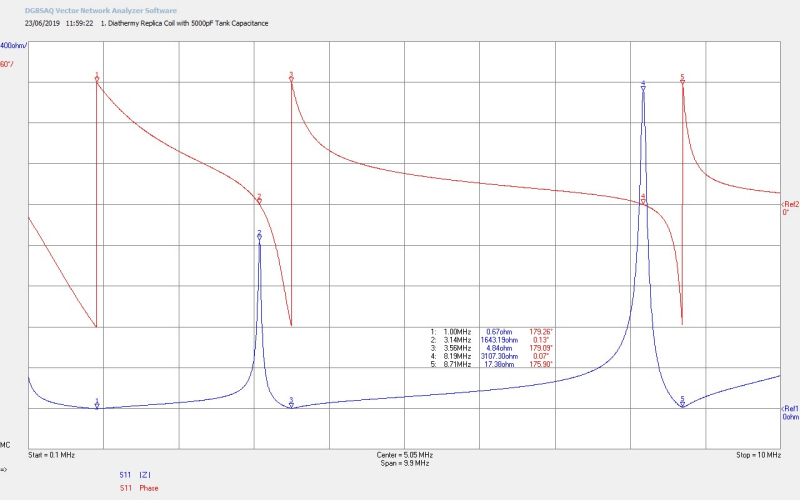
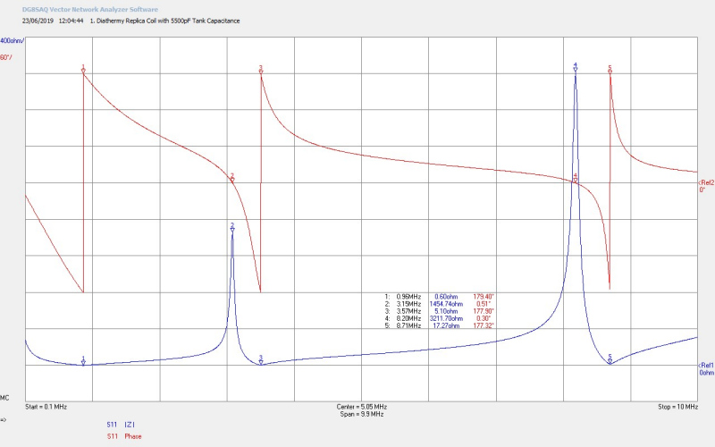
Figures 2 below show the small signal impedance measurements for Z11 up to 10Mc/s at the output of the spark gaps, (with the HV unit disconnected), and then with progressive change of tank capacitance to show the change in tuning, and the optimum match between the primary and secondary of the diathermy replica (DR) unit:
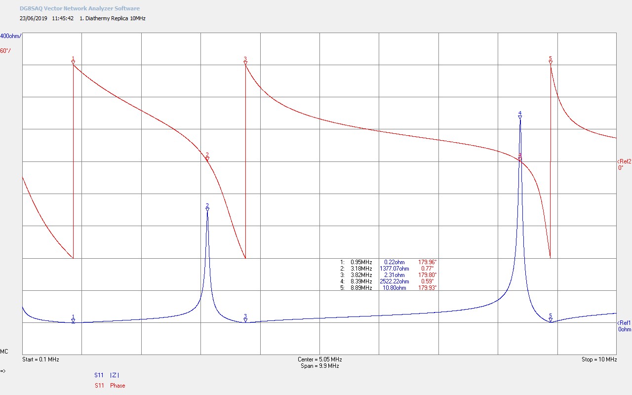
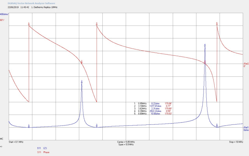
Fig. 2.1 Input impedance Z11 for the DR over a bandwidth of 10Mc/s, showing the primary resonance at M1, the Tesla secondary fundamental resonant frequency at M2, and the second harmonic at M4.
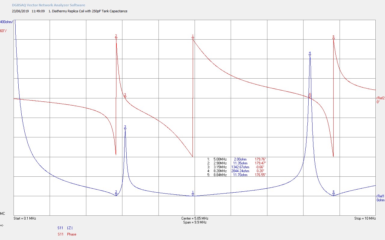
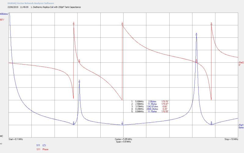
Fig. 2.2 The primary series resonance M1 has moved to 5.0Mc/s with the tank capacitor reduced to 250pF.
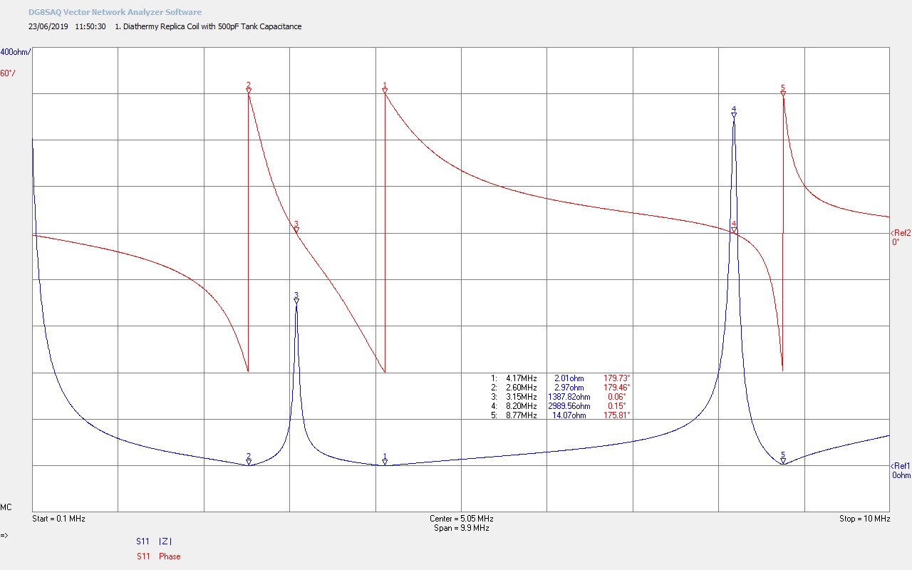
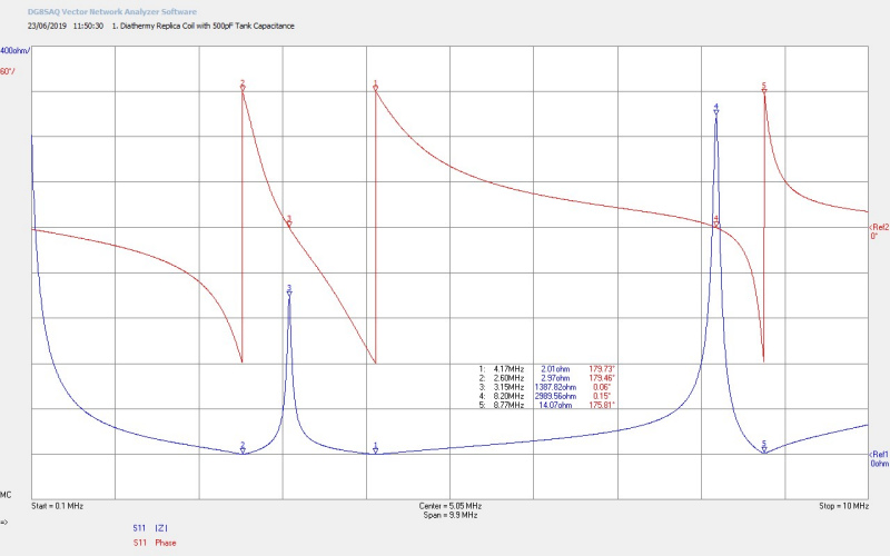
Fig. 2.3 Tank capcitance increased to 500pF shows M1 moving closer to the secondary at 4.17Mc/s.
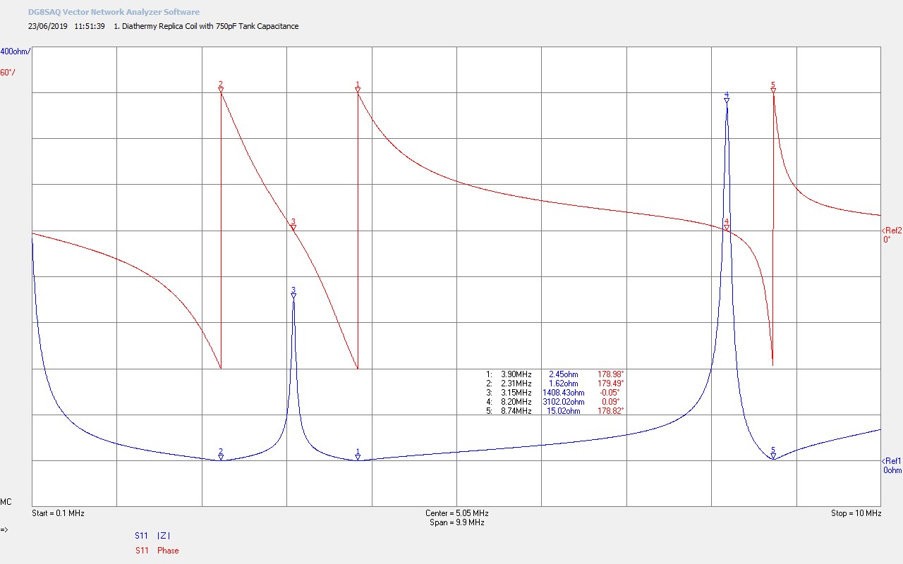
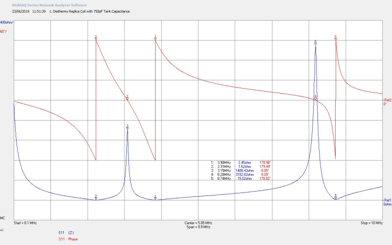
Fig. 2.4 Theoretical optimum tank capcitance achieved at 750pF where M1 and M2 are equally divided around M3, the primary resonance matches the secondary resonance at 3.15Mc/s.
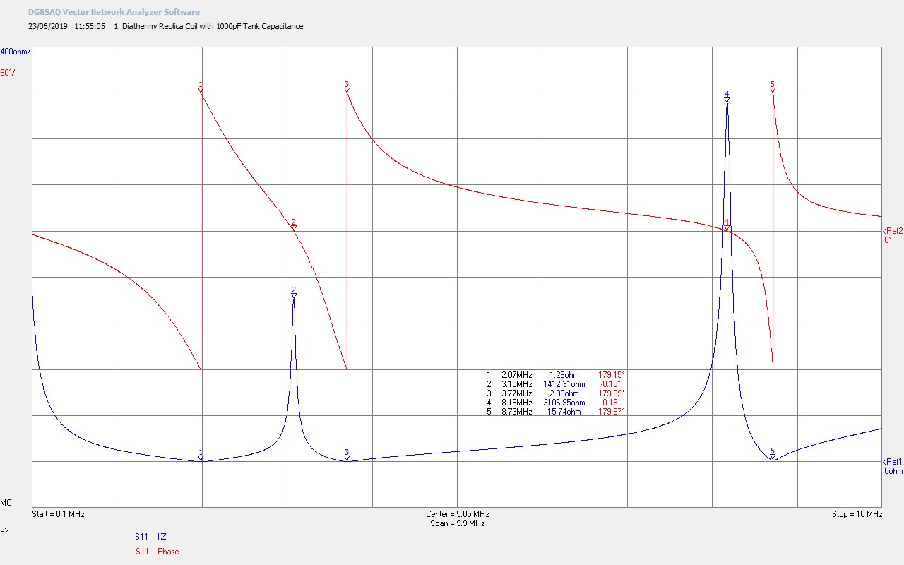
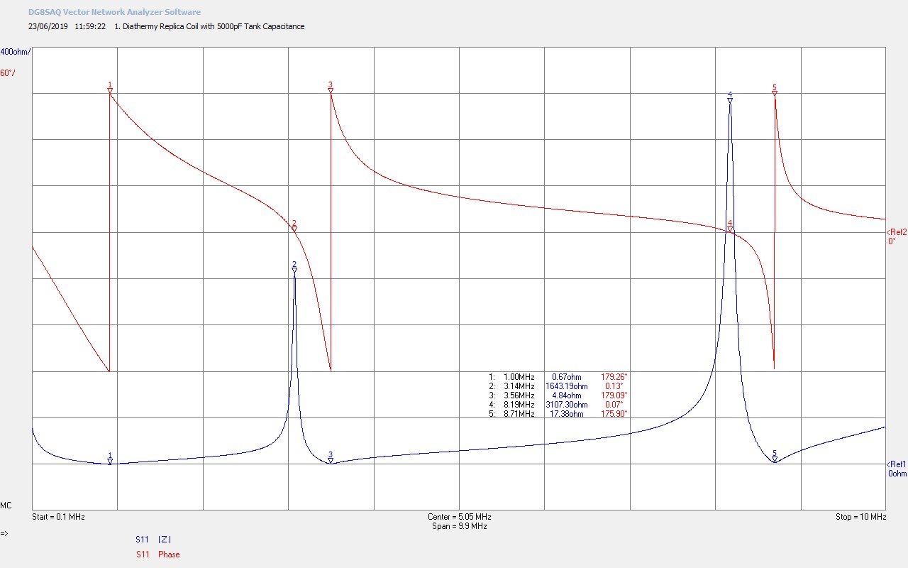
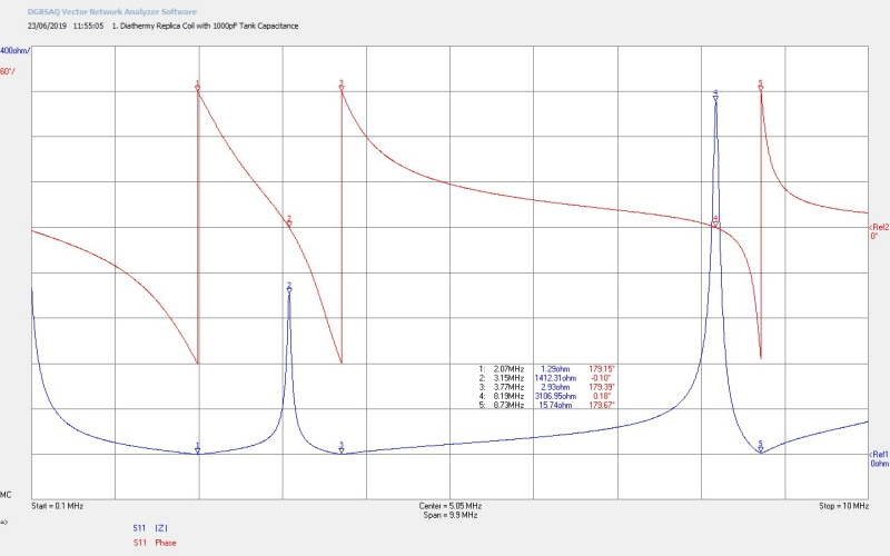
Fig. 2.5 Empirical optimum tank capacitance reached towards 1000pF as the primary resonance at M1 moves away from M2 at 3.15Mc/s. Discharge in the secondary will cause the secondary resonant frequency to drop towards M1, improving the match between the two.
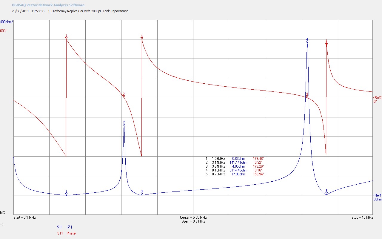
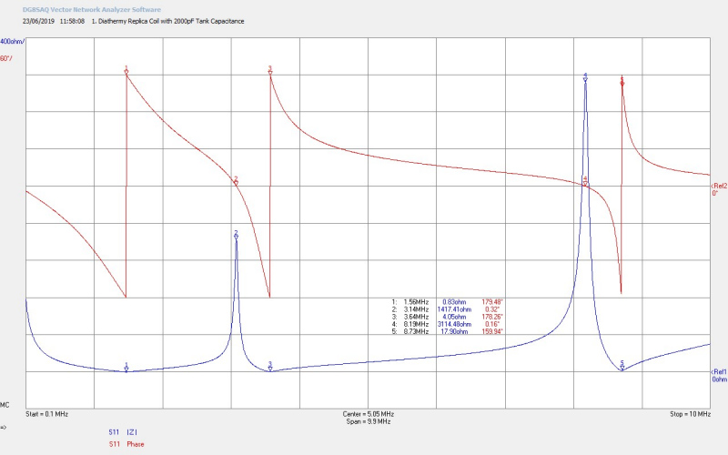
Fig. 2.6 Primary resonance at M1 falling away from the secondary at M2, reducing the match, and hence the power coupled between the primary and secondary.
Fig. 2.7 Primary resonance M1 moving far away from the secondary reducing the coupled power, limiting the secondary currents, and considerably reducing the strength of the secondary discharge.
Fig. 2.8 Effective tank capacitance that brings the response to the non-adjusted response of the DR, where the series primary resonance M1 is at 0.96Mc/s, and the secondary parallel resonance is at M2 at 3.15Mc/s.
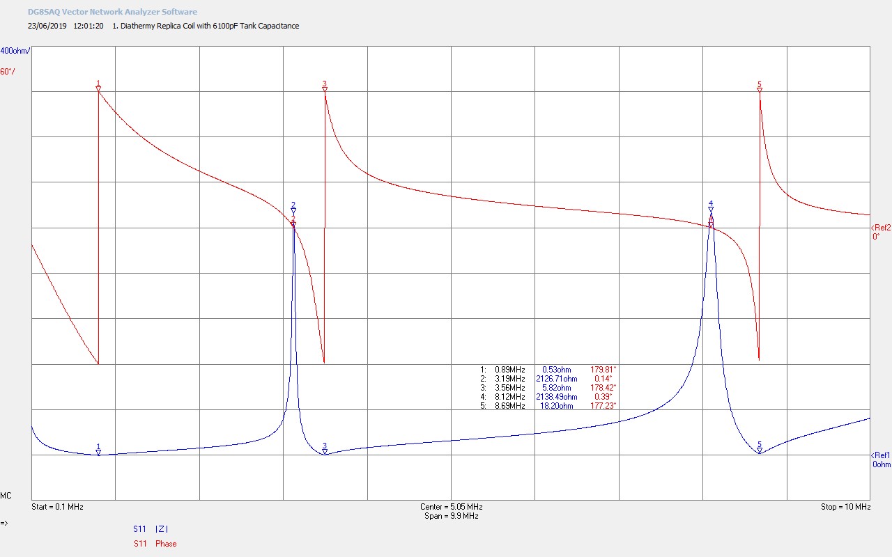
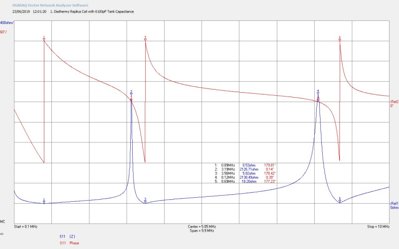
Fig. 2.9 The effective tank capacitance of 6100pF which matches the large signal primary and series resonant frequencies shown in Figures 2.3 and 2.4.
To view the large images in a new window whilst reading the explanations click on the figure numbers below, and for a more detailed explanation of the mathematical symbols used in the analysis of the results click here. For further detail in the analysis and consideration of Z11 typical for a Tesla coil based system click here.
Fig 2.1. Shows the resonant frequencies of the both the primary and the secondary coils in the DR. M1 (marker 1) is the fundamental resonant frequency FP of the primary, showing the 180° phase change that takes place at the resonant frequency, and the minimum impedance point of a series resonance where |Z| has no reactive components and only reflects the electrical resistance of the primary coil. FP at 950kc/s is a result of the series combination of the primary coil inductance and resistance LP and RP, and the combined two series banks of tank capacitors CP, and any stray L and C that result from the inter-connecting wires and boundaries to the surrounding medium. RP ~ 0.22Ω is low and indicates a good primary coil size and material, which will enable larger discharge currents to flow, facilitating stronger oscillations to be coupled to the secondary, and an improved power transfer between the primary and secondary coils.
M2 shows the fundamental resonant frequency of the secondary FS = 3180kc/s, and M3 the frequency at which a 180° phase change takes place FØ180 = 3820kc/s. As is normal for a secondary coil where there is considerable distributed resistance across the coil end points FS and FØ180 do not occur at the same frequency, and the parallel resonance formed between LS and the distributed capacitance CS set the fundamental resonance of the coil at M2. When electrical energy is coupled to the secondary from the primary the coil will resonate at the frequency indicated at M2.
Where required FS can be made to more closely match FØ180 by adding additional loading capacitance to the open end (top-load) of the secondary coil. This is a very common practice for large discharge Tesla coils, (designed for powerful streamers), where metal toroids are added as a top-load and add additional loading capacitance bringing FS much closer to FØ180. This also reduces the Q of the Tesla coil and hence is not desirable for experimental coils designed to explore the inner workings of electricity.
It should be noted that the fundamental resonant frequencies of the primary FP and secondary FS do not correspond at the same frequency, as would normally be expected and tuned for a spark gap driven Tesla coil arrangement. Normally to gain maximum power transfer between the two coils their resonant frequencies will be arranged to be the same through tuning of the primary, (Lp or Cp dependent on the type of coil, how it is constructed, and with what materials). This means that in the DR case less power than optimum is coupled to the secondary, and hence the strength of any discharges from the output of the EHT terminal are reduced. Since the DR is based on the original HGF specifications it is conjectured that this may have been desirable for medical diathermy applications to restrict the strength of the EHT discharges by deliberately mis-matching the resonance of the two coils.
The second harmonic of the secondary FS2 occurs at M4 and M5. If the primary is tuned closer to M4 then the secondary coil will resonate at FS2 = 8390kc/s which represents the second odd harmonic of the secondary wire length, 3λ/4. The parallel resonance at M4 is noted to be quite strong, with a similar Q to the fundamental, indicating that the secondary could have a better response to impulse currents generated in the system. Impulse currents due to there very sharp, high energy, wide frequency band, excite a wide range of resonances within a typical Tesla coil system. The ability for the system to respond to such impulse currents largely depends on the overall Q of the coil’s harmonics. The series resistance at M5 becomes the limiting factor in how much power can be coupled to harmonics of the coil, and has risen considerably from M3 from 2.3Ω to 10.8Ω.
It can be noted from part 1 that the designed Fλ/4 (FØ180) was simulated for the coil dimensions, turns, and construction as 3806kc/s which is only ~ 0.4% error from that measured in the small signal Z11 analysis at 3820kc/s, (Fλ/4 occurs at M3, and is based on the λ/4 length of the coil when one end of the coil is at a low impedance, and the other at a high impedance).
Fig 2.2. Shows the dramatic effect of reducing the total tank capacitance CP down to 250pF. The marker number for the primary M1 has been kept the same despite the order of the coil resonances changing across the 10Mc/s band. M1 the series resonant frequency of the primary FP has now moved right up to 5Mc/s, which has also resulted in a reversal of M2 and M3 so the that FS is now above FØ180 at 3150kc/s. The effect of moving the primary resonance point, through the tuned primary tank CP, is to mis-match the primary and secondary resonances the other way, increase the effective series resistance of the primary coil resonance from 0.22Ω to 2.0Ω, but to leave the actual fundamental resonance frequency of the secondary FS with only a ~1% change from 3180kc/s to 3150kc/s. Increasing M1 to between the fundamental FS and the second harmonic FS2 has also had a more dramatic impact on the frequency of the second harmonic, reducing it from 8390Kc/s to 8200kc/s, a change of ~ 2.3%.
It should be noted that the dependence of FS and FØ180 to tuning in the primary is dramatically different for the flat coil parallel tuned, and the cylindrical case series tuned. For the flat coil, parallel resonance tuned, FØ180 remains more constant with changes in CPP, and is almost exclusively effected only by the secondary wire length, whereas FS, and its harmonics FSN, vary very widely based on changes in CPP. In the cylindrical coil, series resonance tuned, the dependence reverses and FØ180 varies very widely with changed in CPS , whilst FS, and its harmonics FSN, remain more constant with changes in CPS. This emphasises the need for the correct choice in the type of secondary coil used for any specific experiment (e.g. flat, cylinder, equal ratio etc.), and also the correct choice of primary tuning mechanism, (parallel or series). The characteristics and differences, and hence the choice for specific types of experiments, for each of these different coil configurations will be considered and reported in more detail in subsequent posts on the cylindrical coil.
Fig 2.3. Here CP is now increased to 500pF and M1 starts to move downwards again towards the secondary FS. In this case FP is approaching the point of optimum match where the primary and secondary are equally split between the centre point. With CP = 500pF the match is still a little high where the primary is resonating at a frequency above the secondary.
Fig 2.4. Here CP is now increased to 750pF and M1 and M2 are now equidistant either side of FS at M3. Once again FS has not really changed significantly and is still at 3150kc/s. This point of match is in principle the most optimum match between the primary and secondary coils, where maximum power can be transferred between the two coils.
In practise and for maximum streamers it is usually preferred to operate this form of cylindrical Tesla coil, where FP is slightly below FS, due to FS falling when a discharge (streamer) occurs. The discharge causes a change in the impedance of the secondary coil reducing its resonant frequency FS, bringing FS during discharge to an optimum match with the primary, allowing maximum power transfer from the tank through to the secondary discharge.
In experiments to explore the displacement and transference of electric power, where it is preferable not to produce discharge streamers (dissipating the energy of the system through transference), the optimum match where FS = FP is the preferred condition. This is where the Q of the system is maximum, and the continuity between the electric and magnetic fields of induction between primary and secondary are optimum, which in turn ensures the maximum dynamic stability, and best departure point from a system in equilibrium.
Fig 2.5. Here CP is now increased to 1000pF, FP is slightly below FS, (observed in the larger gap between M1 and M2, than M2 and M3), which is around the best empirical match for a Tesla coil designed for maximum discharge as discussed in the previous section.
Fig 2.6. Increasing CP to 2000pF starts to move FP more rapidly away from FS, the match between the primary and the secondary is reducing, and hence the coupled energy is also reducing.
Fig 2.7. At CP = 5000pF FP is now approaching the DR design of Fig 2.1, FP = 1000Kc/s, and FS remains mainly constant at 3140kc/s, only having changed ~ 0.3% as CP changes in the range 250pF – 5000pF.
Fig 2.8. At CP = 5500pF FP is now very similar to the DR design of Fig 2.1, however FS has not yet increased slightly to match the 3180kc/s in Fig 2.1. CP is somewhat different to the expected ~ 7200pF of the two Cornell Dubiller tank capacitor banks which in combination is 6 capacitors of 47nF in series.
Fig 2.9. Here CP has been increased to 6100pF, where FP matches to the large signal primary resonant frequency observed during the time domain experiments shown below in Fig 3.3 at 895kc/s. FS which is now 3190kc/s has finally moved slightly away from the previously stable 3150kc/s, but notably is now closer to the DR design of Fig 2.1, and also the large signal secondary resonant frequency of 3214kc/s shown in Fig 3.6 below.
Overall the small signal Z11 analysis of the spark gap generator reveals a wealth of detail in understanding how this generator is characterised in the frequency domain, and how best to match the primary tank capacitance to obtain different operating points according to the purpose of the experimental system.
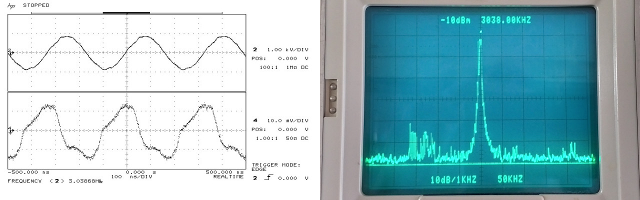
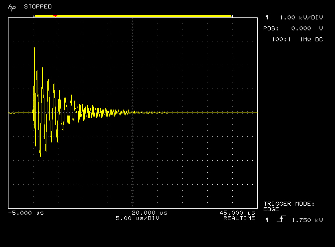
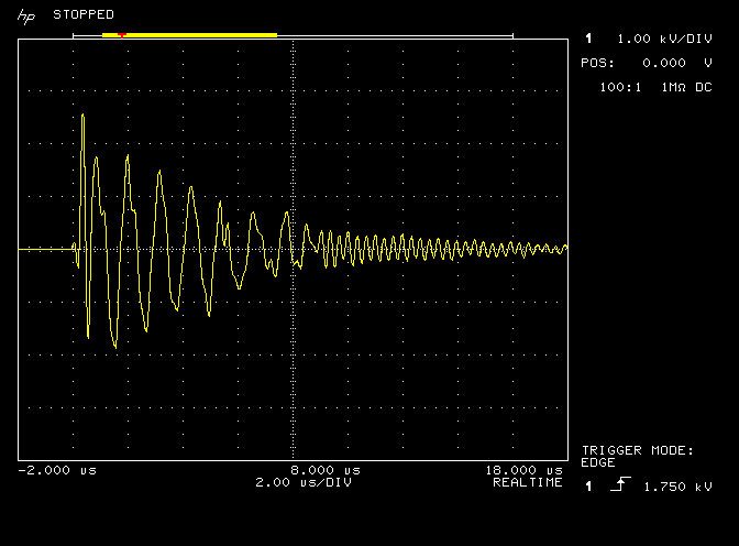
Figures 3 below show the large signal time domain waveforms of the spark gap generator as measured from the low output tap, and illustrate the different stages of the spark discharge burst both in the primary and secondary coils of the generator. The spark gap generator was being run at an input power of 300W, (monitored using a Yokogawa WT200), which was kept constant throughout the measurement of both Figures 3 and 4. Output waveforms were measured using a Pintek DP-50 high voltage differential probe, (max. 6.5kV up to 50Mc/s), which was connected to a HP 54542C oscilloscope to observe and record the output waveforms.
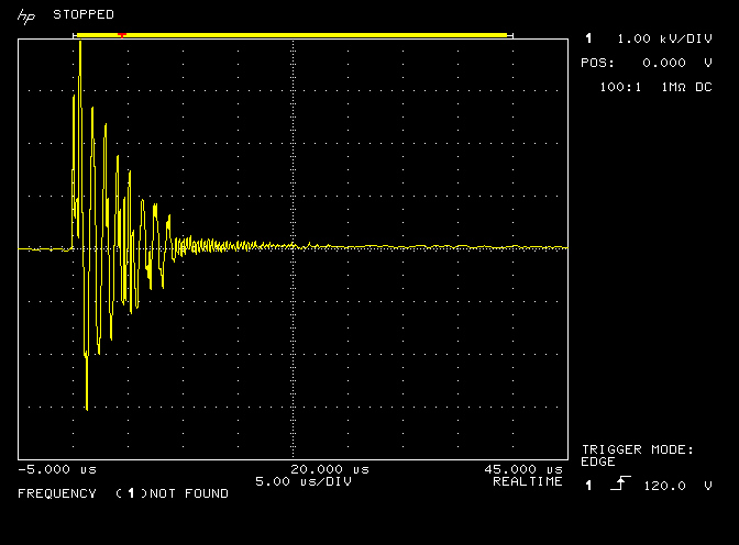
Fig. 3.1 DR burst discharge and ring-down in the primary and secondary, measured at the primary low (L) output tap.
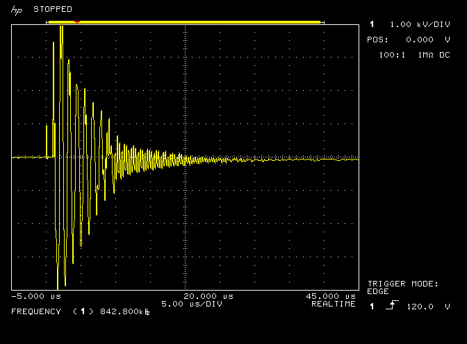
Fig. 3.2 Time magnified DR burst discharge and ring-down in the primary and secondary, measured at the primary low (L) output tap.
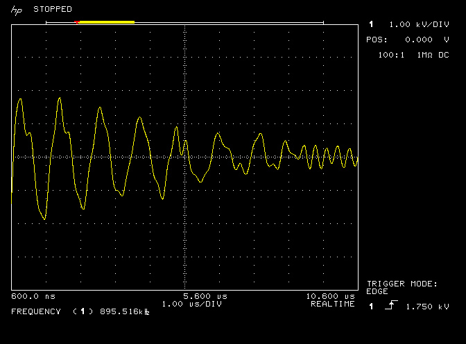
Fig. 3.3 Time magnified DR burst showing the oscillations in the primary coil at a resonant frequency of 895kc/s, and after a phase change the start of the ring-down oscillations in the secondary.
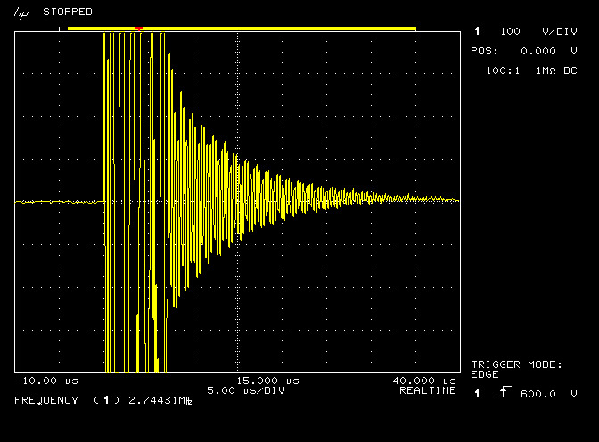
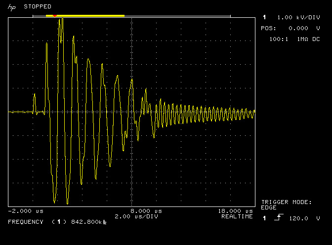
Fig. 3.4 Amplitude magnified DR burst showing the oscillations in the primary and secondary coil, and illustrating the ring-down envelope in the secondary after the spark discharge has finished in the primary.
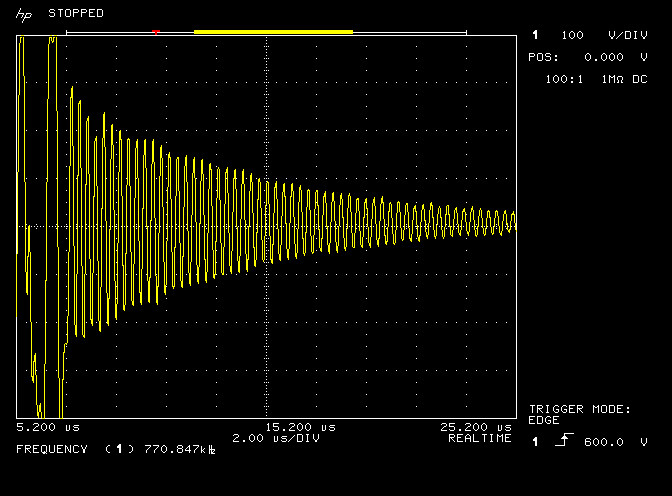
Fig. 3.5 Delayed and time magnified DR burst showing the last oscillations in the primary and the ring-down of the secondary coil.
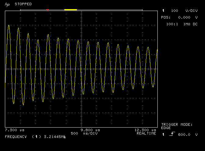
Fig. 3.6 Time and amplitude magnified DR burst showing the oscillations of the secondary coil at 3.21Mc/s.
To view the large images in a new window whilst reading the explanations click on the figure numbers below:
Fig 3.1. Shows the burst waveform measured at the low output tap of the DR. The vertical amplitude scale is 1kV/div, and the horizontal timebase is 5µs/div. The oscilloscope was adjusted to acquire the burst in single-shot mode, triggering at a low to high transition of 1.75kV, where the output delay was adjusted to coincide the trigger to the start of the second full horizontal division. The burst waveform is formed of three major sections, where the first is right at the point of triggering and always involves a very sharp impulse type transition, the second a ring-down of specific frequency based on an exponentially decaying oscillation in the primary coil of the DR, and the third, a ring-down of another specific frequency on an exponentially decaying oscillation in the secondary coil of the DR.
The first section occurs right around the moment of initiation of discharge of the spark gap, and includes a very sharp impulse transition, where the amplitude of this impulse can be many times more than the nominal tension of the high voltage supply. This section requires more detailed capture and measurement with a more sophisticated experimental setup, and will therefore be considered and reported in a subsequent post. Here it is sufficient to understand that there is an impulse like start to the spark discharge, which only lasts for a very brief moment around the initiation of the discharge, and produces very narrow and sharp amplitude spikes at the very beginning of the output burst.
The second section is established right after the spark discharge has started, and the energy stored in the two tank capacitor banks is being discharged in the primary circuit. Before the spark discharge is initiated the tank capacitors are charged by line frequency alternating current supplied by the output of the high voltage supply, where the charging circuit is formed by the high voltage transformer connected through the tank capacitors to the primary coil. When the tension across the output of the transformer has risen above the combined breakdown voltage of the spark gap unit, the spark discharge begins and the impedance across the spark gap suddenly changes from an open-circuit to almost a short-circuit.
The inputs to the primary tank capacitors are now shorted together by the spark and the tank capacitors discharge their stored energy rapidly through the primary coil. The resonant primary circuit formed by the tank capacitors in parallel with the primary coil cause the discharge to oscillate at a frequency defined by LPCP, and this oscillation lasts until the tank capacitors are completely discharged. How rapidly the capacitors discharge at the resonant frequency and the magnitude of the oscillating currents generated in the primary circuit is dependent on the series resistance presented by the primary circuit, which should ideally be as low as possible, and in the case of the DR was measured in Fig 2.1. to be ~ 0.2Ω.
The oscillating currents in the primary during the spark discharge of the tank capacitors, couple through induction to the secondary of the Tesla coil in the DR, or more clearly, a sudden change to the prior equilibrium state of the electric and magnetic fields of induction energy in the system result in energy being accumulated in the secondary coil. In the third section of the burst discharge this accumulated energy in the secondary transforms to oscillating currents at a frequency defined by the secondary resonant circuit LSCS. The secondary oscillating currents decay exponentially in the secondary coil, (assuming no streamer discharge from the secondary), according to the series resistance presented in the secondary circuit. These secondary oscillating currents again couple through imbalance in the electric and magnetic fields of induction back to the primary circuit, where they can be observed in the output waveform as the third section of the ring-down, which dominates the output when the second section oscillations have become sufficiently small.
The complete burst waveform lasts for about 20µs before decaying to less than 1% of its initial amplitude. Bursts are initiated each new cycle of the line frequency, so for UK standard line input at 50Hz to the high voltage supply, a burst is generated every 10ms, (2 per cycle), or at a frequency of 100Hz.
Fig 3.2. Here the horizontal timebase has been reduced to 2µs/div which accordingly magnifies the burst discharge showing more detail in the first, second, and third sections. In the second section and with careful observation it can be seen that the oscillation is not a pure sine wave, it is actually the oscillating currents of the primary circuit with the smaller oscillations of the secondary super-imposed over the top. The super-imposed secondary currents are not easily discernible in the second section because the amplitude of the oscillation in the primary circuit are large.
As these primary oscillations decay away, and after ~ 8µs, a phase change in the output occurs and the secondary oscillations now dominate the output with an envelope that carries the small decaying primary oscillations. In other words the overall burst waveform is a superposition of the oscillating currents in both the primary and the secondary in both sections two and three, where one or the other can be clearly observed based on the energy stored in the respective resonant circuit, and that coupled forward and backward through the inter-action of the two coils.
Fig 3.3. Here the horizontal timebase has been further reduced to 1µs/div and the waveform buffer delay adjusted so that section two dominated with the primary oscillations fills almost the entire trace. The transition to the third section can be seen in the last two divisions of the trace. With section two the main focus of this trace the monitored average frequency of trace 1 can be seen to be 895kc/s which is FP, the fundamental resonant frequency of the primary circuit. The amplitude of the primary oscillations is almost 4kVpk-pk at the beginning of the section, and has decayed after 8µs to ~ 1kVpk-pk.
Fig 3.4. Shows the discharge burst in magnified amplitude against the original horizontal timebase rate. The amplitude has been magnified by a factor of 10 from 1kV/div to 100V/div which illustrates clearly the transition to the third section where oscillations in the secondary coil, coupled back into the primary coil, are a superposition of the both the primary and secondary oscillations, and hence the envelope of the waveform in the third section appears similar to an amplitude modulated waveform. Note: the indicated frequency on this trace is not accurate as it is calculated by averaging together sections 2 and 3, and cannot be considered to be the fundamental frequency of the secondary coil.
Fig 3.5. Here the discharge burst is magnified both in vertical amplitude and in the horizontal timebase, and illustrates more clearly the decay and envelope of the secondary oscillations.
Fig 3.6. Here the discharge burst is further magnified in the horizontal timebase and delayed into the third section of the discharge burst, which shows the monitored average frequency of trace 1 to be 3214kc/s which is FS, the fundamental resonant frequency of the secondary coil.
The large signal time domain waveforms have also revealed a wealth of detail about the operating characteristics of the spark gap generator, showing the nature and characteristics of the oscillating output waveform, and with well-defined sections that can be corresponded to the frequency domain properties measured in Figures 2. The results have also shown impulse like characteristics in the first section of the waveform, that certainly require more investigation and more detailed measurement to clarify if they relate to, and contribute to, the conjecture of underlying displacement phenomena within electricity.
Figures 4 below show a comparison on the same vertical and horizontal scale of the low, medium, and high output taps. It can be seen that the amplitude of the output increases with each successive tap, consistent with the geometry of the primary/Oudin arrangement of the coils.
Fig. 4.1 DR burst discharge and ring-down in the primary and secondary, measured at the primary low (L) output tap.
Fig. 4.2 Increased amplitude DR burst discharge and ring-down measured at the primary medium (M) output tap.
Fig. 4.3 Maximum DR burst discharge and ring-down measured at the Oudin coil high (H) output tap.
Fig. 4.4 Magnified DR burst discharge and ring-down measured again at the Oudin coil high (H) output tap.
The low tap produces about 4kVpk-pk initial output, the medium tap 8kVpk-pk, and the high Oudin tap ~ 11kVpk-pk but at considerably reduced current. The medium output tap has been determined to be the best tap for driving TMT experiments, and other experimental apparatus suited to the exploration of the displacement and transference of electric power, where there is high output tension combined with stronger oscillating currents.
Summary of the generator results and conclusions so far:
1. The results and measurements for the spark gap generator correspond well between the frequency and time domain, and give a good insight into how this type of generator works, and the type of output that can be generated. The generator presented in parts 1 and 2 were initially used to confirm the experiments and results of Dollard et al.[1,2], before being applied widely to my own research into the inner workings of electricity.
2. This generator has been proven to be reliable and robust and can sustain indefinitely output powers of 1.5kW, and short bursts over 2kW with the appropriate connections and arranged loads.
3. This generator transforms the low frequency alternating currents of the line input, into high frequency oscillating current outputs, combined with considerably increasing the tension of the output.
4. Analysis, of particularly the time domain results, indicates a first section in the discharge burst that may include impulse currents and effects that are conjectured to involve displacement events. This section requires more detailed measurement and analysis, and will be reported in subsequent posts.
1. Dollard, E. & Lindemann, P. & Brown, T., Tesla’s Longitudinal Electricity, Borderland Sciences Video, 1988.
2. Mackay, M. & Dollard, E., Tesla’s Radiant Matter Replication, 2013, Gestalt Reality
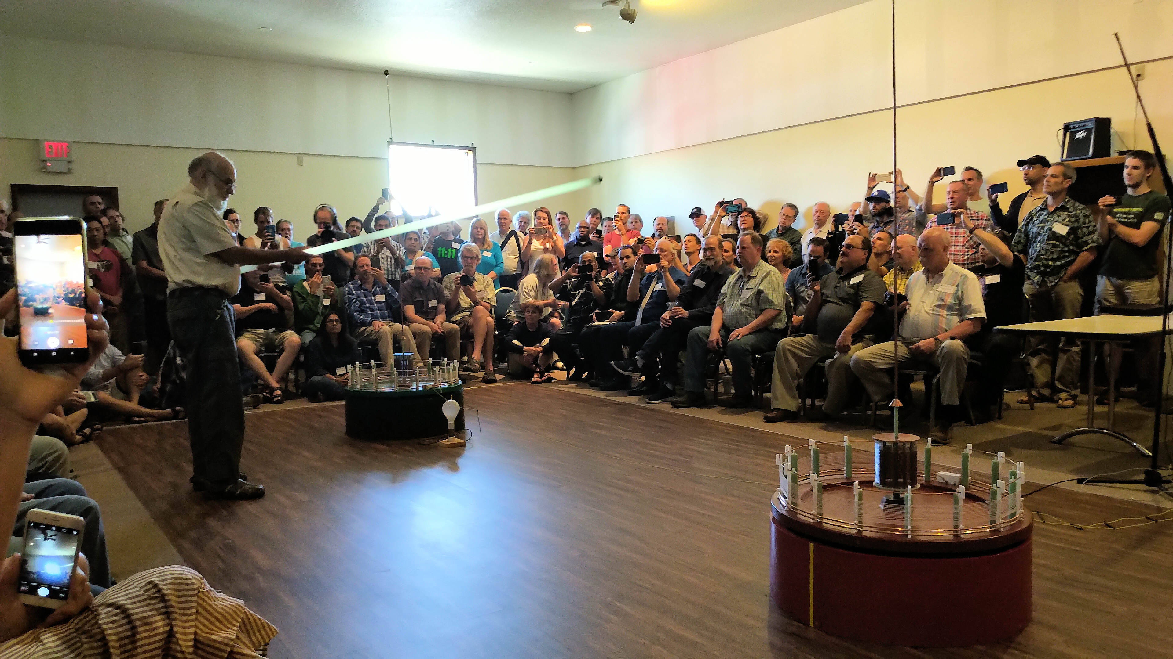
ESTC 2019, the Energy, Science, and Technology Conference[1], included a presentation and working demonstration by Eric Dollard on Tesla’s Colorado Springs experiment[2] (TCS), which is available through A & P Electronic Media[3,4]. Due to unforseen circumstances relating to the demonstration co-worker, the generator for this experiment was unavailable after the demonstration for additional experimentation, investigation, and follow-up demonstrations. In agreement with Eric Dollard I suggested that the spark gap generator from the Vril Science Multiwave Oscillator Product[5], (MWO), could be adapted, tuned, and applied to the Colorado Springs experiment, and in order to facilitate ongoing investigation and experimentation throughout the conference period. What follows in this post is the story of how this successful endeavour unfolded in the form of videos, pictures, measurements, and of course the final results.
The first video below shows highlights from the endeavour, video footage was recorded and supplied by Paul Fraser, and reproduced here with permission from A & P Electronic Media.
The second video below shows highlights from the impedance measurements part of the endeavour, video footage again by Paul Fraser, and by Raui Searle.
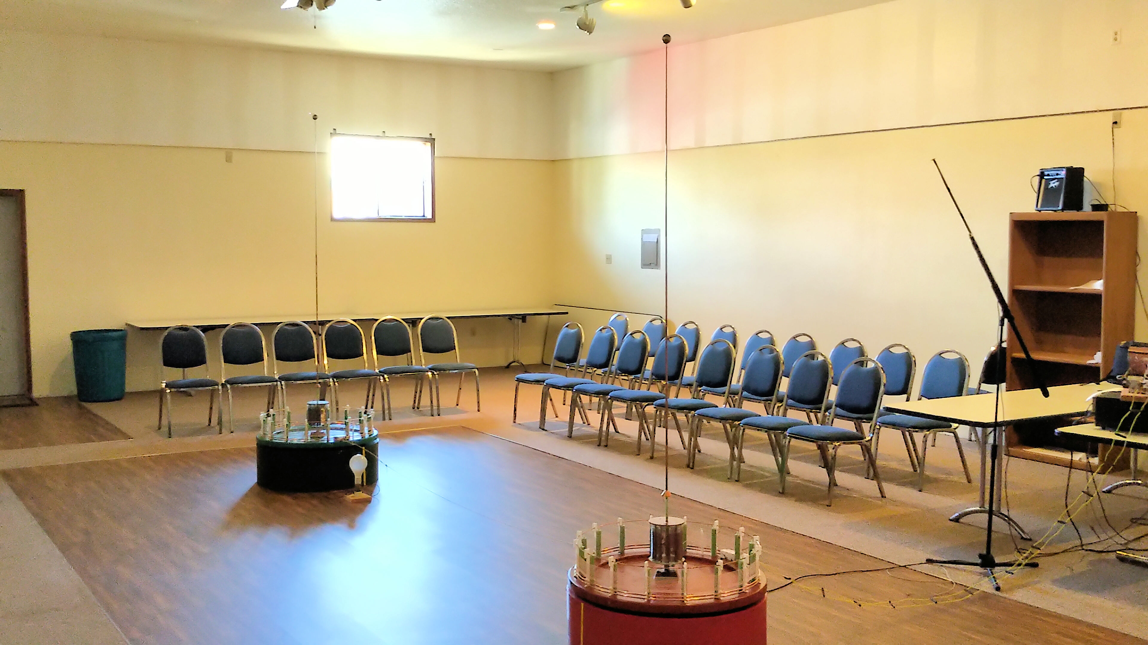
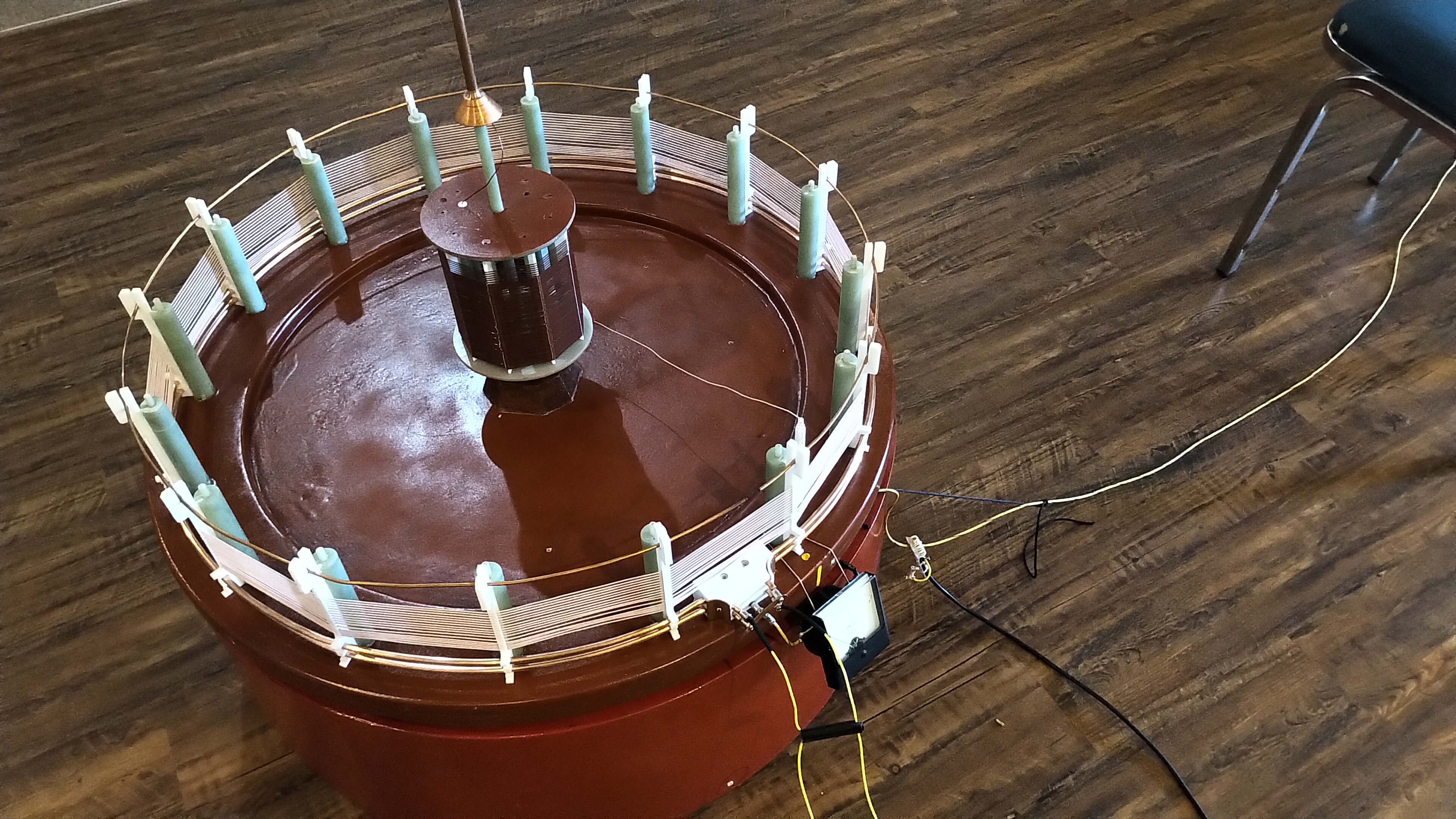
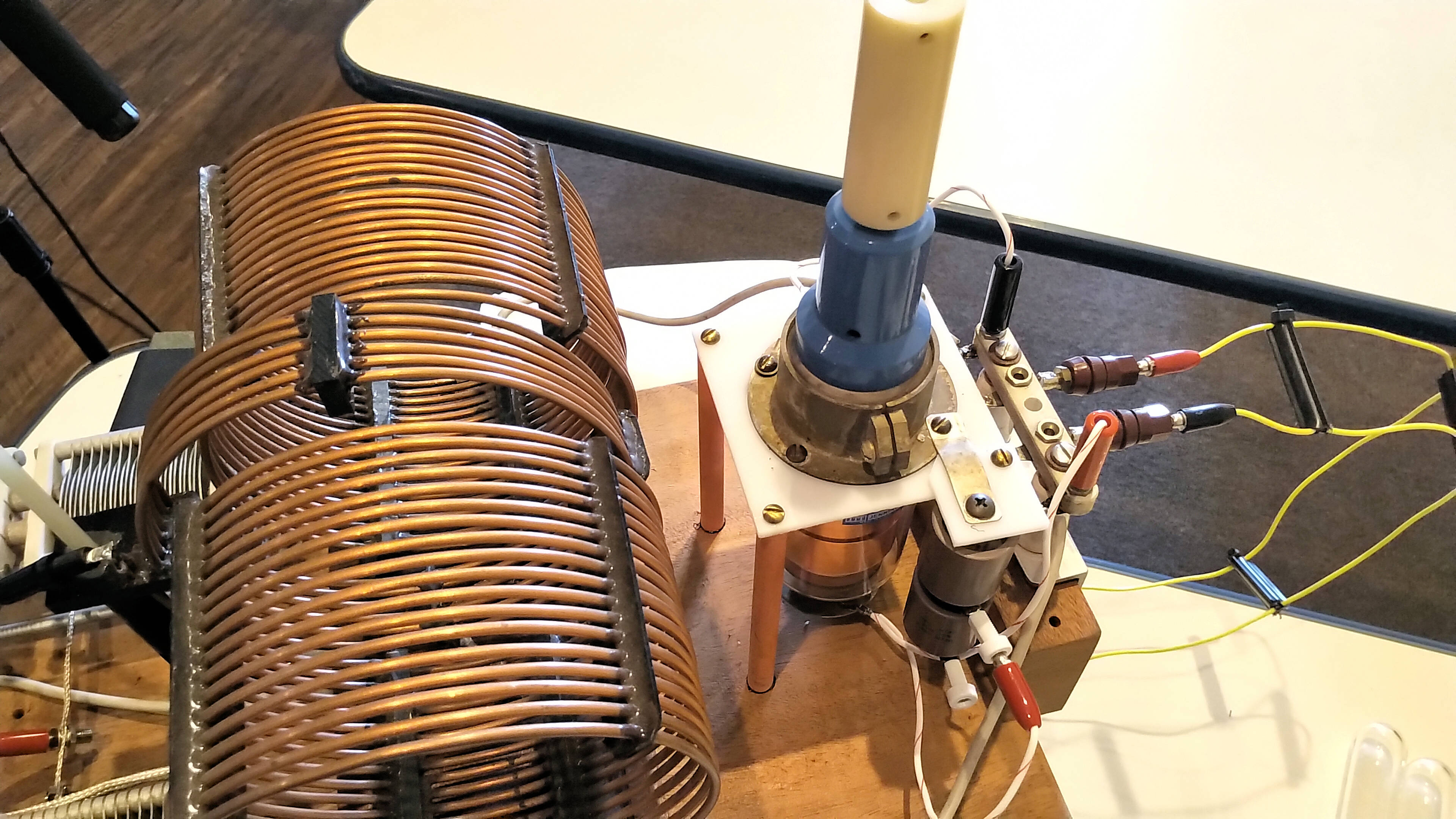
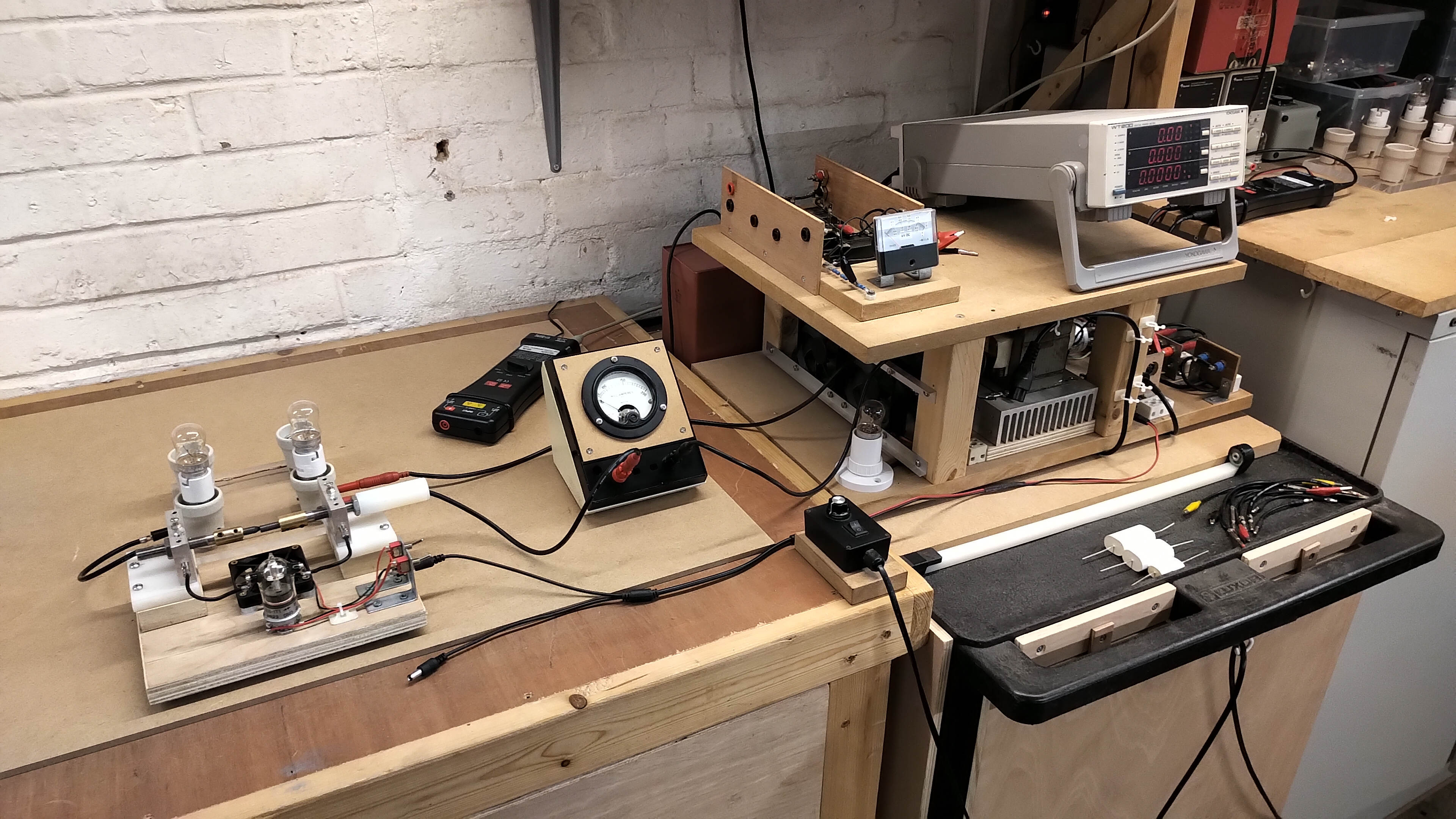
Figures 1 below show a range of pictures of the original transmitter and receiver setup from Eric Dollard’s TCS demonstration, including the generator used to power the experiment, and key results from the original demonstration. The red “transmitter” coil (RTC) was subsequently modified after the demonstration, (secondary coil re-wound, and with a single copper strap primary), in order to work well with the MWO spark gap generator. The green “receiver” coil (GRC) was left un-modified for the purpose of the endeavour, although it could be fine tuned using the extra coil telescopic extension. Ultimately for on-going experiments using the MWO generator, the GRC would be re-wound and adapted to more closely match the RTC.
Fig. 1.1 The coil arrangement for the TCS demonstration by Eric Dollard, showing both the red transmitter coil and the green receiver coil.
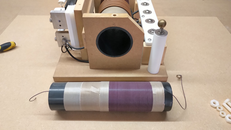
Fig. 1.2 The red transmitter coil showing the general arrangement of the primary, secondary, and the extra coil.
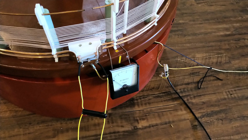
Fig. 1.3 The generator is connected to the primary via a balanced transmission line, and the secondary is connected to the green receiver coil via an rf ammeter.
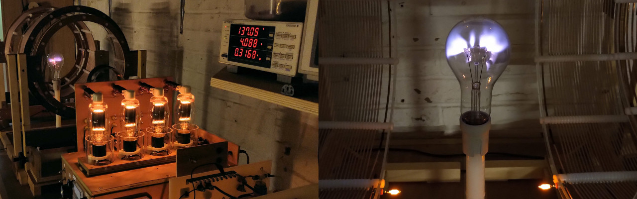
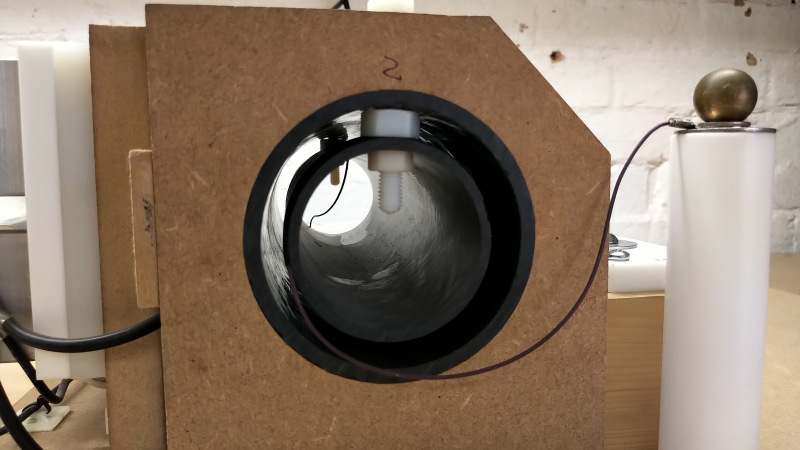
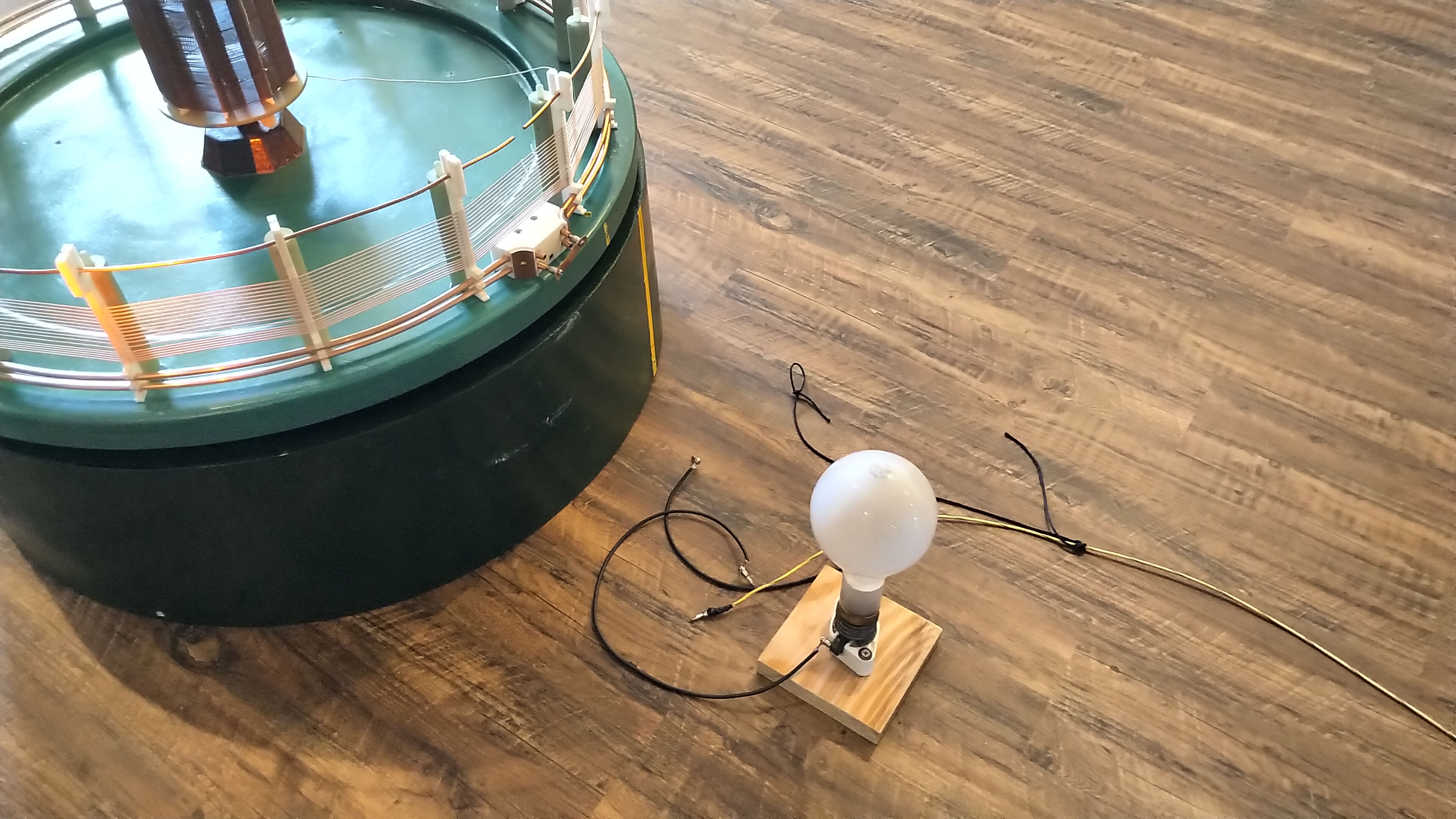
Fig. 1.4 The receiver load is a 500W incandescent light bulb, connected to the primary of the receiver coil. The receiver is connected by a single wire to the transmitter.
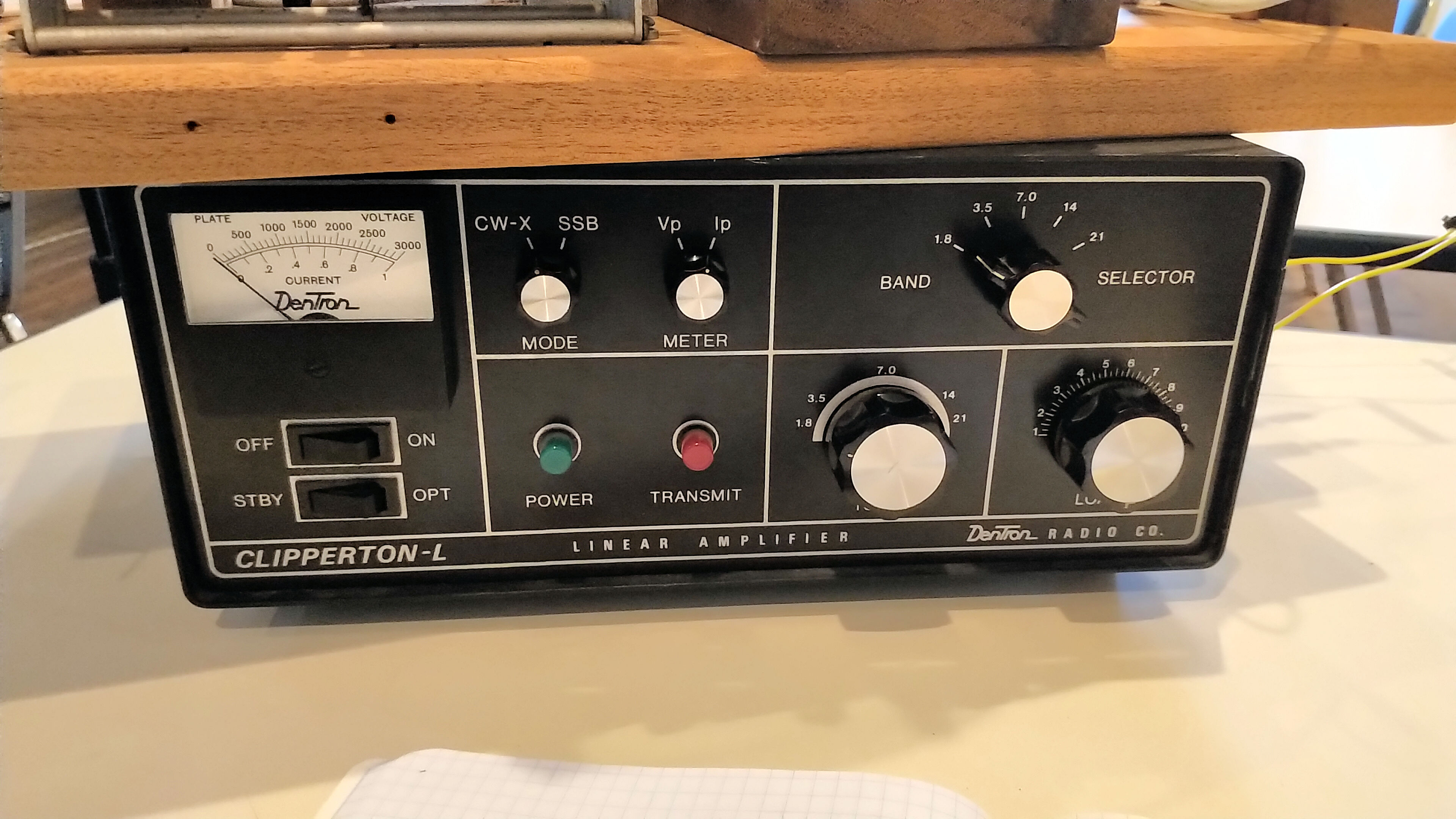
Fig. 1.5 The linear amplifier is a 1000W Denton Clipperton-L, and is connnected to the red transmitter coil via a matching unit.
Fig. 1.6 The linear amplifier output matching unit is in itself a tuned resonant transformer, which matches the output of the amplifier on the 160m band to the much lower impedance of the primary in the MW band.
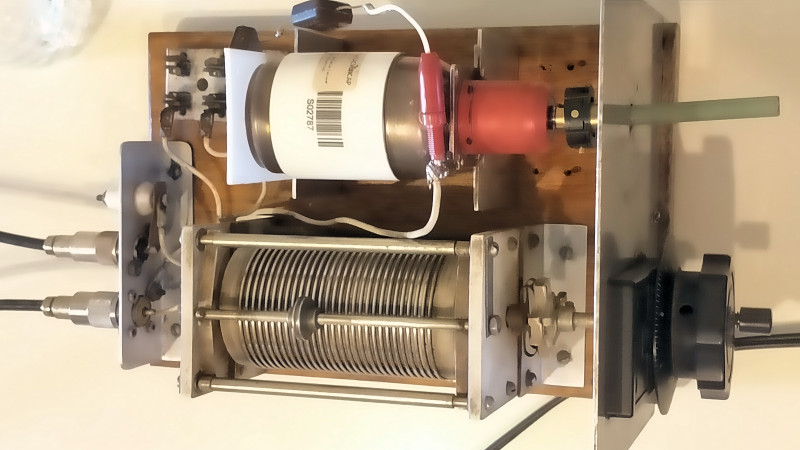
Fig. 1.7 The output of the matching unit is via variable high voltage tuning capacitors in parallel with the output coil.
Fig. 1.8 The input to the matching unit is via a balanced transmission line to a tuned vacuum capacitor, and in parallel with the twin series connected input coils.
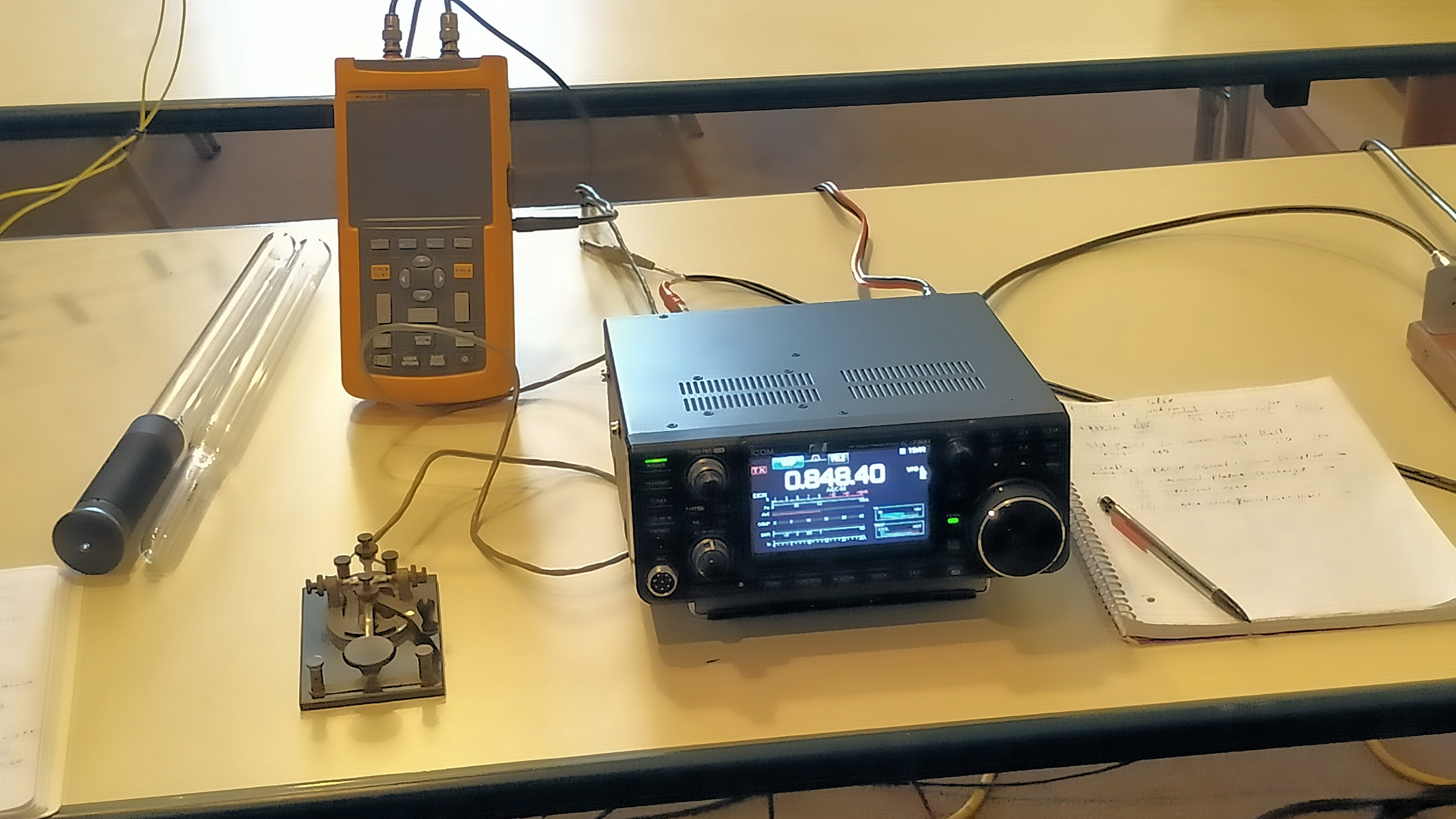
Fig. 1.9 The signal source for the linear amplifier is from an ICOM 7300 amateur radio receiver, modified to transmit on the MW band at 848.4kc/s.
Fig. 1.10 The Denton linear amplifier has no matching input network, hence a matching unit is required between the ICOM 7300 transceiver and the amplifier.
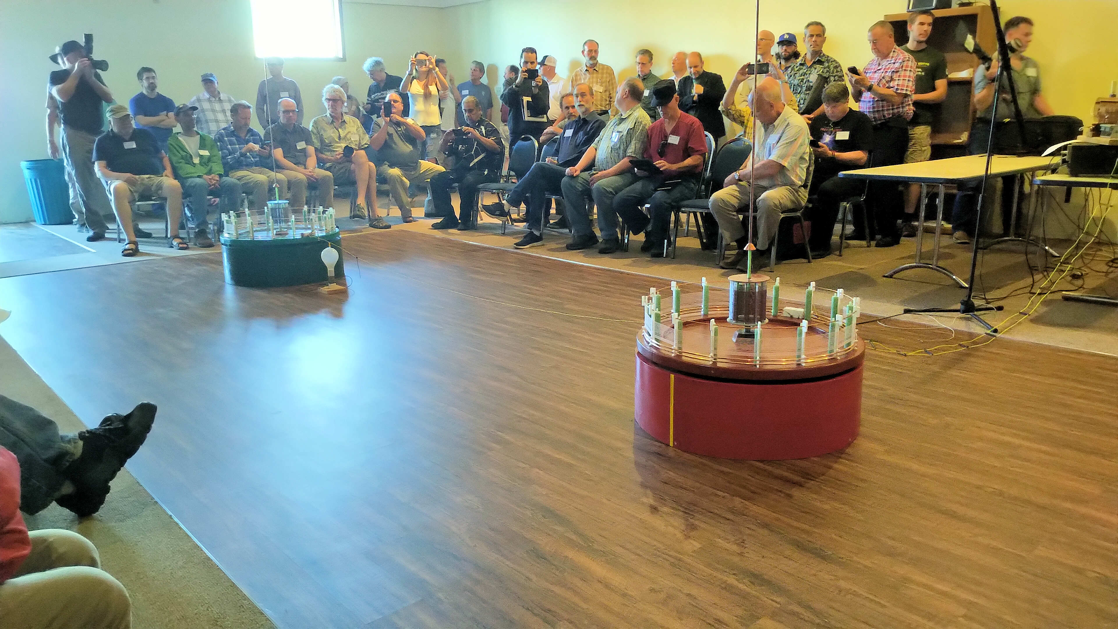
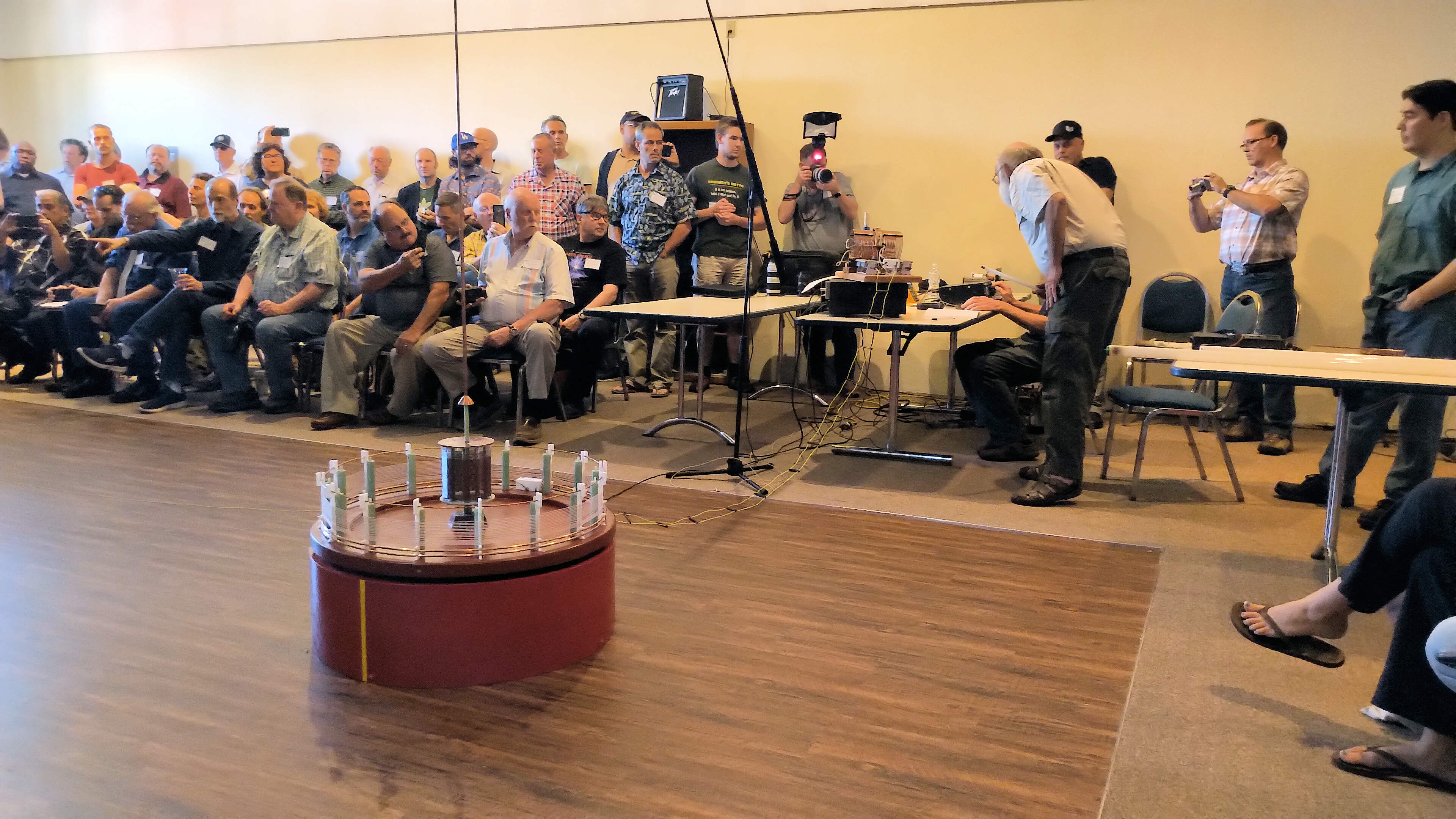
Fig. 1.11 All parts of the system connected together prior to the beginning of the demonstration.
Fig. 1.12 Last minute tuning checks by Eric Dollard prior to turning up the power for music transmission to the green receiver via the MW band.
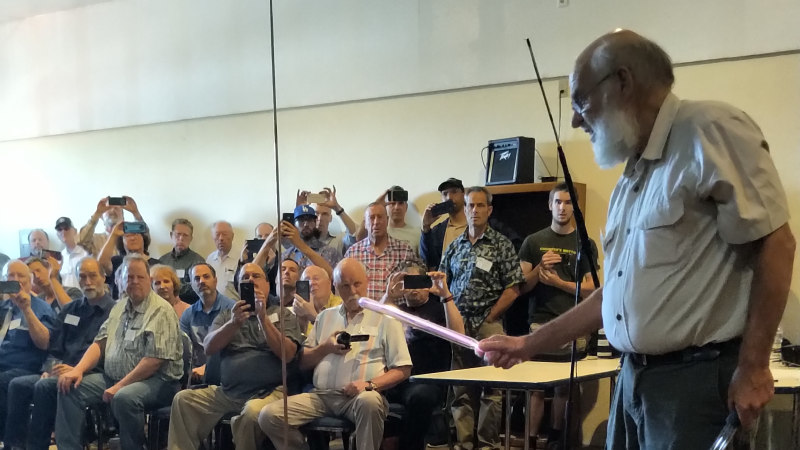
Fig. 1.13 Checking for a null point between the transmitter and the receiver using a domestic flourescent tube to indicate the local electric field strength.
Fig. 1.14 Investigating the field around the extra coil extension using a helium-neon tube.
Fig. 1.15 Transmission of electric power from the transmitter to the receiver via a single wire, and lighting fully a 500W incandescent bulb.
The original TCS demonstration was powered by a 1000W linear amplifier generator being driven at ~ 800W output to light a 500W incandescent bulb at the receiver primary, and where the electric power is transferred between the RTC and GRC by a single wire. The TCS demonstration with both coils fully configured and connected to the generator was tuned to a drive frequency of 848.4 kc/s, as can be seen in fig. 1.9 as the selected frequency of the transceiver.
The transceiver is an ICOM-7300 which must have been modified to allow transmit on all frequencies, a modification that allows a radio amateur transceiver to generate a transmit signal outside of the designated amateur bands. This kind of modification turns a transceiver into a powerful bench top signal generator, with full modulation capabilities, and matched output powers from the transceiver alone of up to 100W in the MF and HF bands (300kc/s – 30Mc/s). 848 kc/s is in the MW (MF) radio broadcast band, and amplitude modulation is well suited here for the transmission of voice and music signals, as was also demonstrated in the original experiment.
The ICOM transceiver is connected via a matching unit to the Denton linear amplifier. This specific brand and model of linear amplifier has no matching unit at its input, which is why external matching is required from the ICOM 50Ω output to the lower impedance Denton input. The passive matching unit is shown in fig. 1.10, and also in the schematic of fig. 2.1.
The Denton Clipperton-L is a linear amplifier using 4 x 572B vacuum tubes with a band selected matching unit at its output, and a total output peak voltage of ~ 500V. The lowest band provided internally for matching at the output of the amplifier is the HF 160m band at ~ 1.8Mc/s. The much lower MW signal at 848kc/s would need additional matching and balancing between the amplifier output and the input to the primary of the RTC, (the output of the amplifier is an unbalanced feed e.g. coaxial, whereas the connecting transmission line and the primary are better fed with a balanced feed). The amplifier passive matching unit is shown in figures 1.6 – 1.8, and is also shown in the schematic of fig. 2.1.
The various different experiments conducted in the original demonstration included the following:
Fig 1.13. Shows Eric Dollard finding the null electric field region between the RTC and GRC, and using a 6′ domestic fluorescent tube light.
Fig 1.14. Shows Eric Dollard testing the field surrounding the RTC extra coil extension top load, using a helium-neon gas filled tube.
Fig 1.15. Shows single wire transmission of electric power, and fully lighting a 500W incandescent light bulb at the primary of the GRC.
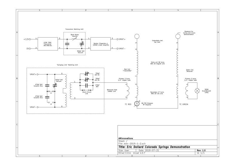
Figures 2 below show the schematics for both the linear amplifier generator and coil arrangement for Eric Dollard’s original TCS demonstration, and a second schematic for the TCS experiment retune using the MWO spark gap generator. The high-resolution versions can be viewed by clicking on the following links TCS Demonstration, and TCS Retune.
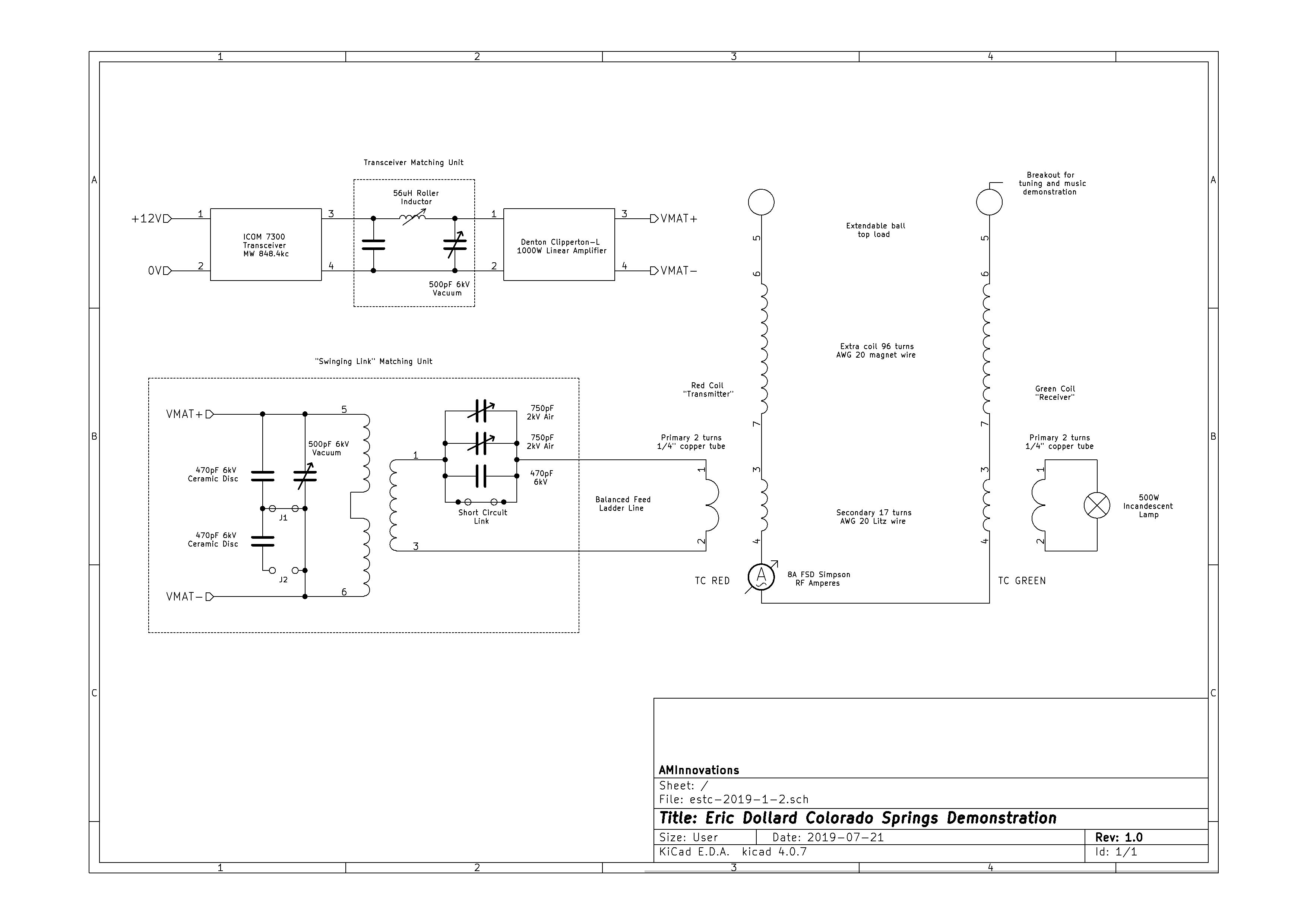
Fig. 2.1 Schematic diagram for the TCS demonstration by Eric Dollard, showing the generator, matching units, and coil arrangements.
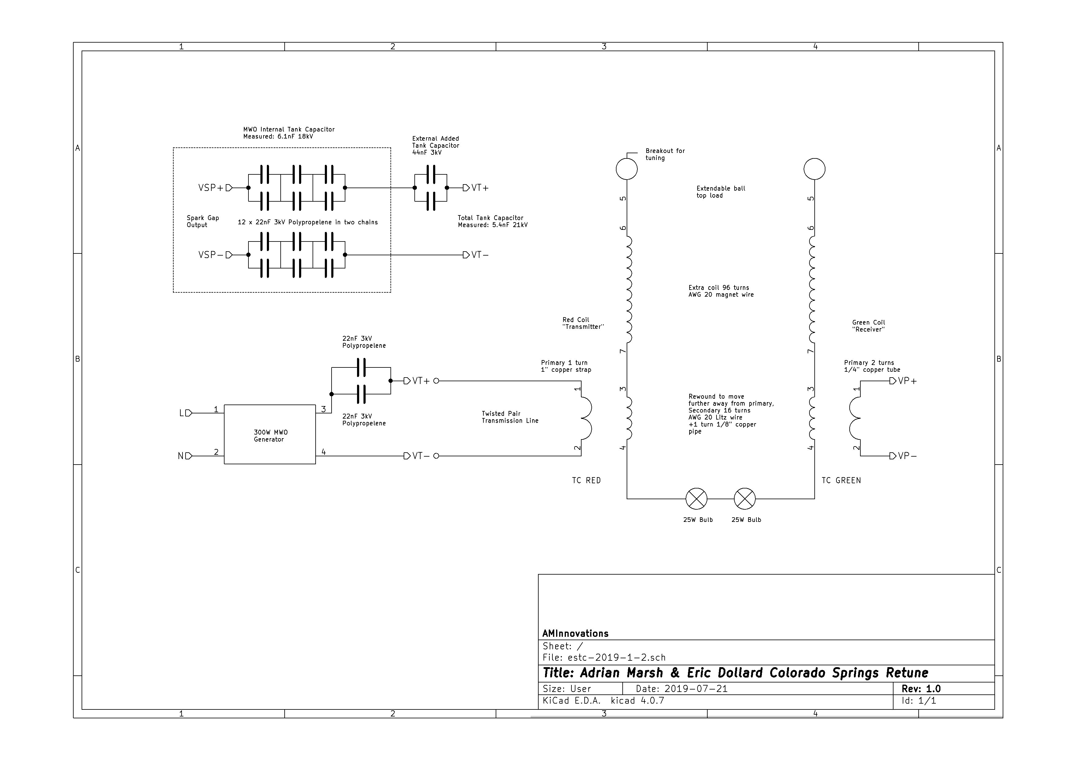
Fig. 2.2 Schematic diagram for the TCS retune by Adrian Marsh & Eric Dollard, showing the MWO generator, tuning capacitors, and modified coil arrangements.
Figures 3 below show the small signal impedance measurements for Z11 for the TCS coils, and also the tuning measurements for the coils and spark gap generator together, which were taken throughout the endeavour and used to ensure a well tuned match between the generator and the TCS experiment.
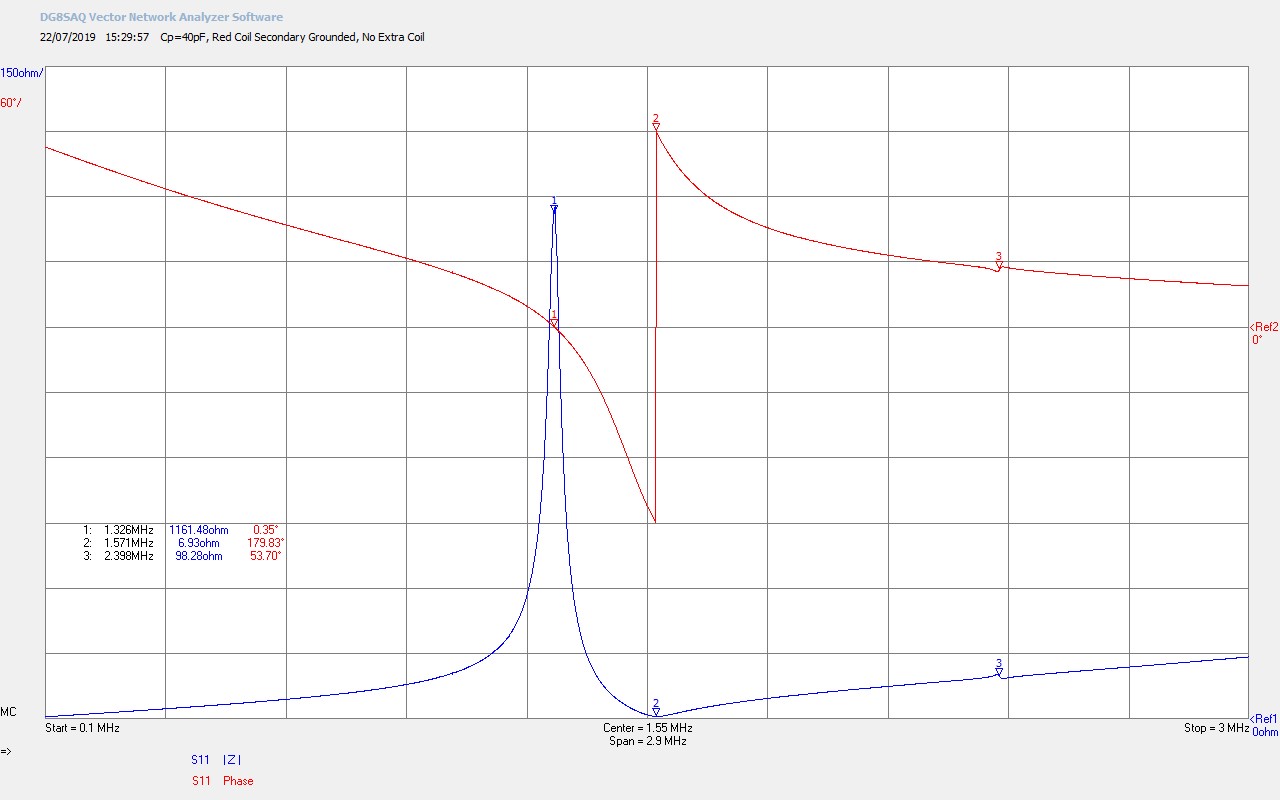
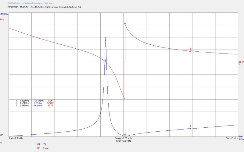
Fig. 3.1 Shows the Z11 impedance for the RTC with the extra coil not connected. The bottom end of the secondary is grounded.
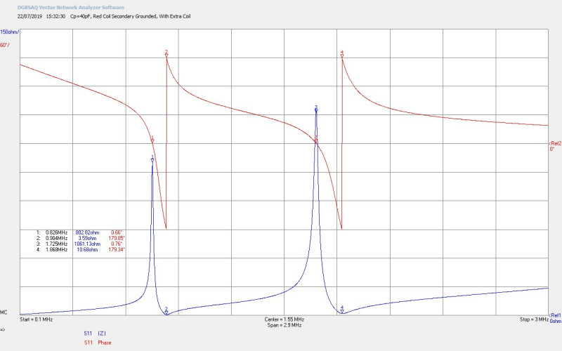
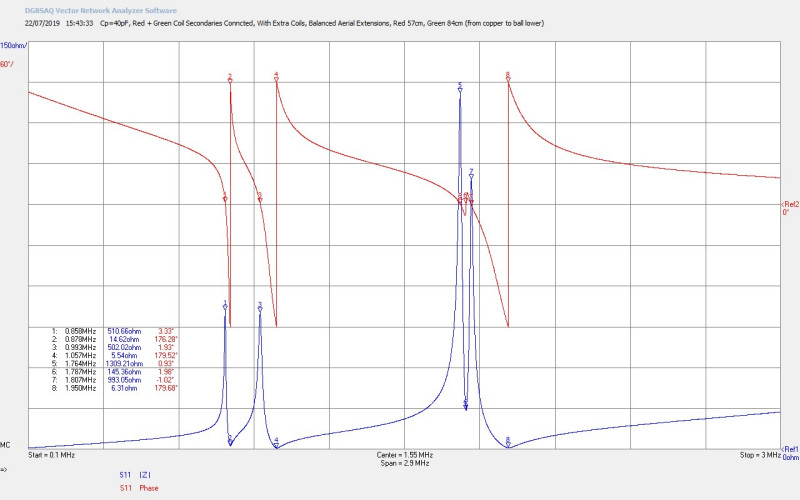
Fig. 3.2 Shows the secondary and the extra coil connected together. The bottom end of the secondary is grounded, and the extra coil extension aerial is fully extended.
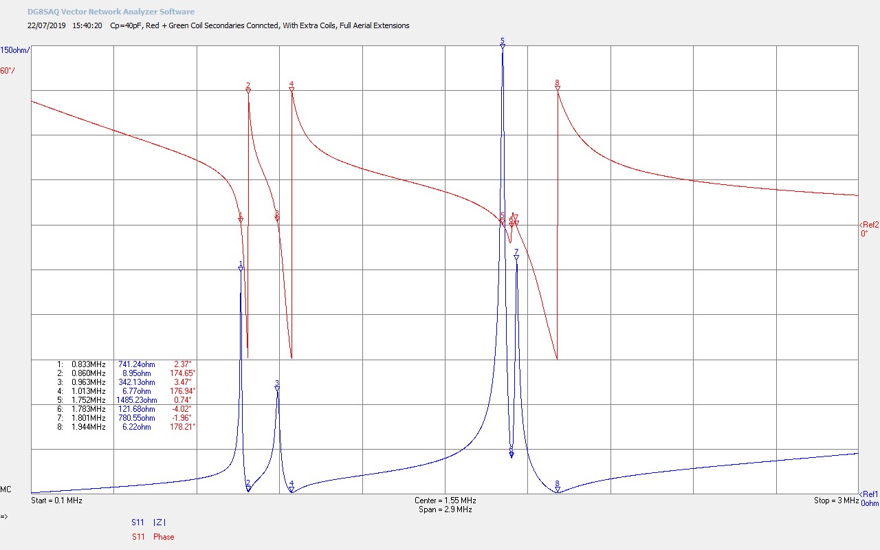
Fig. 3.3 The RTC and GRC are connected by a single wire, and with both extra coil aerial extensions fully extended.
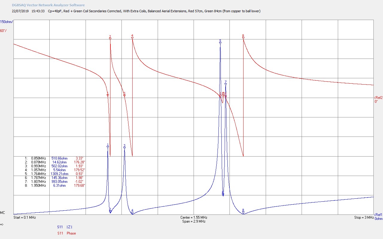
Fig. 3.4 The RTC and GRC are connected by a single wire, and with both extra coil aerial extensions adjusted to balance the impedance of the fundamental resonant frequency.
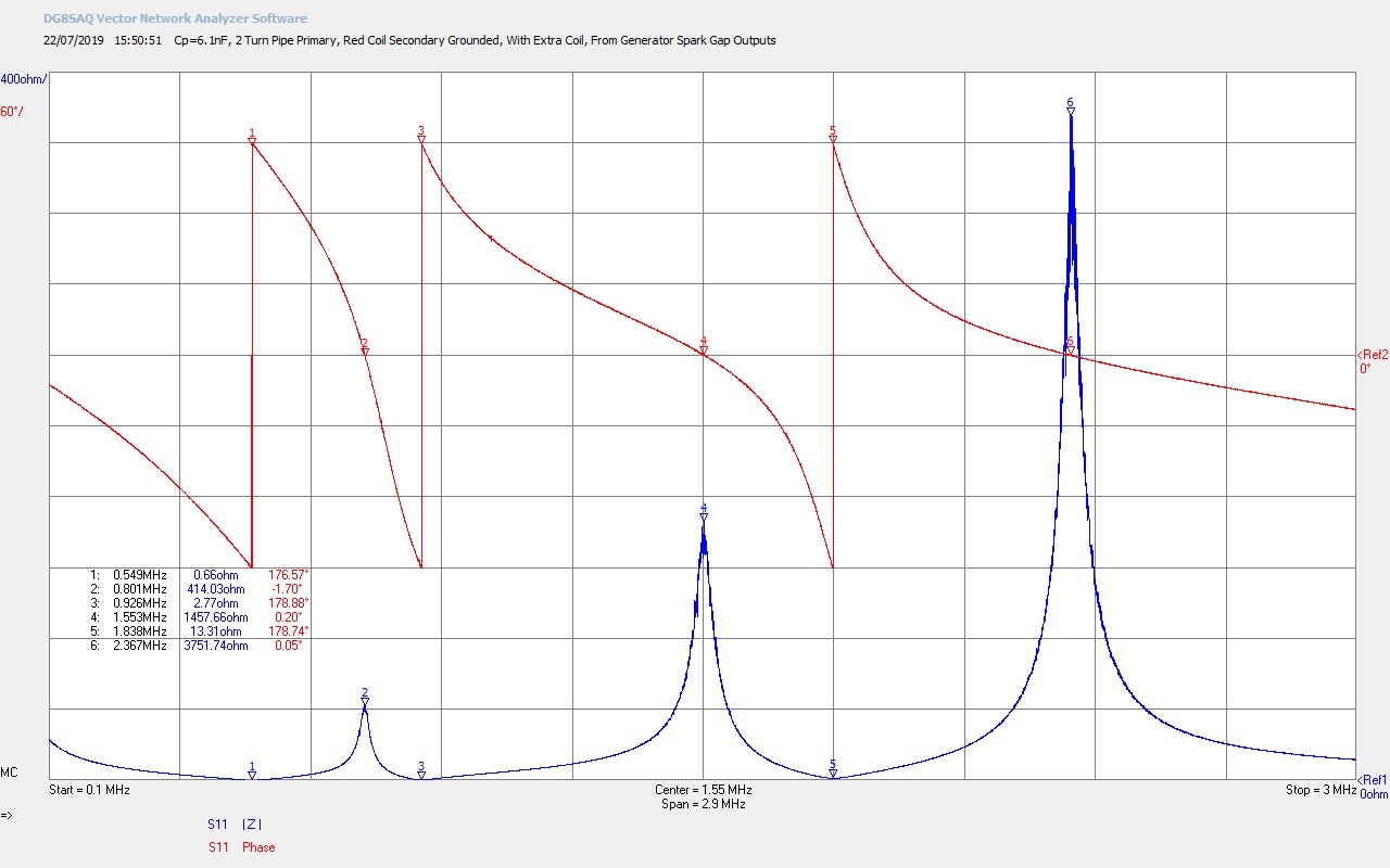
Fig. 3.5 The RTC consisting of a 2 turn copper pipe primary, secondary, and extra coil with extension is connected to the MWO generator at the spark gap outputs, showing the overall tuning from the perspective of the generator.
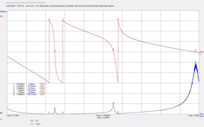
Fig. 3.6 The RTC consisting of a 1 turn copper pipe primary and connected to the MWO generator at the spark gap outputs.
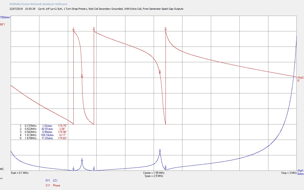
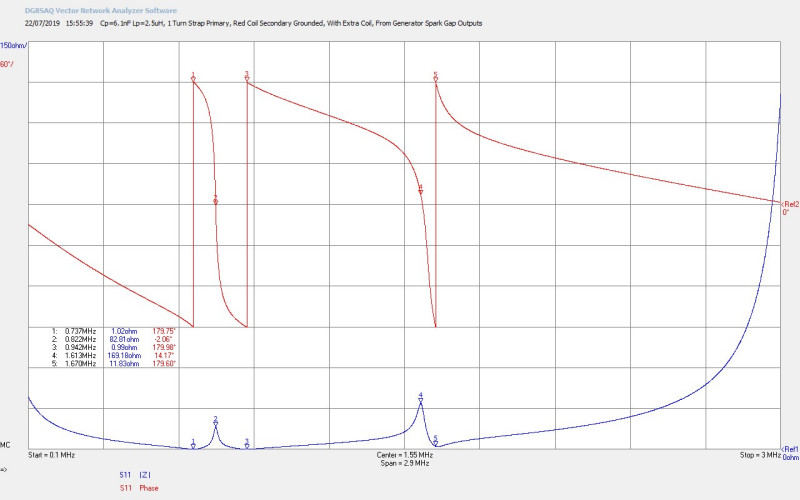
Fig. 3.7 The RTC with a 1 turn copper strap primary connected to the output tuned MWO generator at the spark gap outputs, and showing a clean tuning for the fundamental resonant frequency at 822kc/s.
To view the large images in a new window whilst reading the explanations click on the figure numbers below, and for a more detailed explanation of the mathematical symbols used in the analysis of the results click here. For further detail in the analysis and consideration of Z11 typical for a Tesla coil based system click here.
Fig 3.1. Shows the impedance measurements for the RTC with the secondary grounded, the extra coil disconnected, and where the primary tank capacitance has been arranged to be series CP = 40pf, which puts the primary resonant frequency FP at a much higher frequency and far away from the secondary. This would be the proper drive condition for the original linear amplifier generator (LAG) where FP is not arranged to be equal to FS. For the spark gap generator (SGG) it is necessary to match FP as closely as possible to the combined resonant frequency of the secondary and the extra coil together. The fundamental parallel resonant frequency of the secondary Fs at M1 = 1326kc/s, and as is to be expected with this form of air-cored coil, the FØ180 or series resonant point at which a 180° phase change occurs, is at a higher frequency at 1571kc/s at M2. At M3 = 2398kc/s a tiny resonance is being coupled from the disconnected extra coil which, being mounted in the centre on axis with the secondary, is close enough to have a non-zero coupling coefficient, and hence show some slight resonation reflected into the measurement.
Fig 3.2. Here the extra coil has been reconnected and two resonant features can be noted, the lower from the secondary, and the upper from the extra coil. The effect of the coupled resonance between the two coils with a non-zero coupling coefficient is to push the secondary resonance down in frequency to where the FS at M1 is now at 826kc/s which is very close to the original drive frequency of the linear amplifier generator at 848kc/s. The fundamental resonant frequency of the extra coil, (now in λ/4 mode with one end at a lower impedance connected to the secondary, and the other connected to the high impedance of the extendable aerial), at M3 is now 1725kc/s
Fig 3.3. Here both the RTC and GRC have been connected together to complete the overall system, and where the bottom end of both secondaries are connected together by a single wire transmission line. Both the RTC and GRC have their extra coil adjustable extensions fully extended. It can be seen that both the secondary and extra coil resonant frequencies have been split in two, to reveal four resonant frequencies from the four main coils, 2 in the RTC, and 2 in the GRC. The markers at M1 at 833kc/s and M3 are due to the secondary resonance in the RTC and GRC respectively, and the markers at M5 at 1752kc/s and M7 at 1801kc/s are due to the extra coils. It can be noted that the impedance of the RTC and GRC are not well-balanced the resonance is stronger on the RTC side where |Z| at M1 ~ 741Ω, and M3 ~ 342Ω. During running operation with either the LAG or SGG this would result in more energy stored in the RTC coil, the standing wave null on the single wire transmission line would be pushed away from the RTC and towards the GRC, and less power would be available at the output of the primary in the GRC.
Fig 3.4. Here the lengths of the extra coil extensions have been adjusted to balance |Z| at M1 and M3 at ~500Ω. The RTC extended length was 57cm, and the GRC extended length was 84cm, measured from the copper to aerial join, and to the base of the ball top load. With very fine adjustment, which is very difficult to accomplish, it may be possible to also balance |Z| for the extra coils at M5 and M7. This would result in the ideal balanced and equilibrium state, where the electric and magnetic fields of induction are balanced across the entire system, energy storage is equal, the null point is equidistant between the RTC and the GRC, and maximum power can be transferred between the two coils. In practice, when |Z| for the fundamental secondary resonance is equal, as shown, the overall system can be considered to be well-balanced, and will perform close to its maximum performance. Very slight adjustments to the drive frequency from the generator can then be used to nudge the system into the best overall balance and match. FS at M1 is now 858kc/s which is now close to the original drive frequency of the LAG at 848kc/s.
Fig 3.5. Shows the impedance characteristics of the RTC from the perspective of the SGG. The vector network analyser (VNA) is connected to the outputs of the spark gaps in the generator, so the characteristics include the tank capacitance of 6.1nF and the primary coil, which in this case is 2 turns of 1/4″ copper pipe. It can be seen that the resonant frequency of the primary FP is somewhat below FS as M1 at 549kc/s, and is moving away from M2 and M3. FS has also reduced to 801kc/s at M2 which also shows that the loading in the primary is too much. The inductance of the primary coil, or the tank capacitance, needs to be reduced in order to establish a better match between the generator and the RTC.
Fig 3.6. Here the number of turns of the primary has been reduced to one, which reduces the inductance in the primary resonant circuit with the generator. M1 is now closer to M2 and M3 and the FS has now increased to 819kc/s. The tuning between the generator and the RTC has now swung slightly the other way and the primary is pushing upwards on the secondary characteristics. This state is however a better state of tune than that shown in figure 3.5. It can also be seen that FE for the extra coil is cleaner and less impacted by the primary resonance. Additional fine tuning of the system would ultimately be accomplished by moving one side of the primary connection a certain distance around the circumference of the primary loop, (to form a fractional number of turns in the primary e.g. 1.4), and gain balanced and equidistant spacing for markers M1 and M3 from M2.
Fig 3.7. Here the single turn copper pipe primary has been replaced with a single turn copper strap, which was deemed to present a lower impedance to the generator, and improve the magnitude of the oscillating currents in the primary. In order to further improve the tuning two 22nF 3kV capacitors in parallel (44nF) were added to one of the outputs of the SGG as shown in the schematic of figure 2.2. This reduced the tank capacitance slightly from 6.1nF to 5.4nF. The inductance of the strap was measured to be 2.5uH which combined with the tank capacitance of 5.4nF provides a theoretical lumped element resonant frequency of 1370kc/s. referring back to figure 3.1 it can be seen that FS, the resonant frequency of the secondary, without the extra coil at M1 is 1326kc/s. So the primary circuit tuned and driven at this point has a very close match to the secondary coil, which ensures that maximum energy can be coupled from the primary to the secondary, and then combined with the extra coil, maximum power can be transferred from the generator to the RTC, and ultimately to the GRC when further connected. For the purposes of this endeavour this state of retune was considered adequate for further demonstration and exploration of the Colorado Springs experiment.
The experimental phenomena observed during the operation of the TCS experiment, retuned to work with the MWO generator, can be seen in the first video on this page.
Summary of the endeavour:
The overall endeavour facilitated the demonstration and exploration of tuning and operating the MWO spark gap generator to work with the Colorado Springs demonstration. In the process the RTC primary and secondary needed to be modified for optimum running with the SGG. Throughout the endeavour a wide range of measurements were demonstrated including:
1. Z11 impedance measurements for the series fed secondary and extra coil, for the RTC.
2. Z11 impedance measurements for the primary combined with the secondary, and the exta coil, for the RTC.
3. Combined Z11 impedance measurements for both the RTC and GRC, where the bottom ends of both secondaries were connected together to form a single wire transmission line.
4. Fine tuning of the system by adjusting the wire length of the extra coil extensions, in order to balance |Z11| in the fundamental and second harmonics.
5. Z11 impedance measurements using a computer connected vector network analyser.
The endeavour also facilitated the demonstration and exploration of the following interesting Tesla related phenomena:
6. Single wire electric power transmission.
7. Longitudinal transmission of electric power.
8. Emission of radiant energy pulses from an incandescent bulb.
9. Radiant energy pulses attracting metal to the bulb.
10. Amplification of radiant energy by interaction with a human hand.
11. Transference of electric power between a TMT “transmitter” and “receiver”.
Click here to continue to the next part, ESTC 2022 – Vector Network Analysis & Golden-Ratio/Fractal-Fern Plasma Discharges.
1. ESTC 2019, Energy, Science, and Technology Conference, A & P Electronic Media , 2019, ESTC
2. Dollard E., Preview of Theory, Calculation & Operation of Colorado Springs Tesla Transformer, 2019, EricPDollard
Negative resistance is a feature of the I-V characteristic of a discharge between two electrodes, and if correctly utilised can lead to unusual electrical phenomena within an electrical circuit. In this first part on this topic we explore the I-V properties of the negative resistance (NR) region of a carbon electrode spark gap (CSG), or carbon-arc gap. When the CSG is biased into the correct region, and combined with a switched (non-linear) impetus from the generator, the impedance of the circuit can be seen to reduce from the conventional short-circuit case, increasing the current in the circuit and intensifying the light emitted from an incandescent lamp load.
The negative resistance characteristics of a spark gap where explored and utilised by Chernetsky[1] in order to demonstrate what he called the self-generating discharge (SGD). The SGD is a state of discharge where he claimed that the energy consumed from the generator was reduced, yet the power dissipated in the load was increased, and where the additional energy in the electrical circuit was “inducted” from the surrounding medium, or what is commonly referred to as the Aether[2], a “gaseous” medium that is all pervasive throughout space, and is also considered to extend beyond the physical realm. As such Chernetsky claimed an over-unity (OU) phenomena where the total output power was greater than that supplied to the circuit by the generator. This experiment has been replicated by others, including Frolov[3], and Dawson[4], who also claim to have measured OU output. This sequence of posts investigates these principles, attempts to measure the claimed OU output, and further explore its possible origin. Ultimately the studied phenomena forms part of the continuing central research, of revealing the inner workings of electricity, and hence the displacement and transference of electric power.
When investigating over-unity claims good experimental and scientific method is critically important. I have found many situations where OU has been attributed to unusual phenomena without being supported by good and well measured experimental data. OU most often appears to arise in non-linear systems, which owing to their transient nature are also difficult to measure reliably, especially when output power is to be accurately measured. Input power is usually quite straight-forward to measure accurately as it is supplied by dc sources such as batteries and power supplies, or drawn from the mains utility supply which is a low-frequency sinusoidal input. In these cases electrical instruments can be arranged to accurately determine real and reactive input power.
Where the generator produces a non-linear output through switching, pulses, impulses, or chopping an otherwise dc or low-frequency sinusoid the dissipated output power can become a complex transient, with many high-frequency components, and many different phase relationships within the experimental circuit. When this is combined with high voltage and/or current magnification , multi-resonant elements, different transmission modes both transverse and longitudinal, cavity and termination effects, and hence significantly changing boundary conditions on the dielectric and magnetic fields of induction, the final accurate determination of output power, even with sophisticated instrumentation, is exceedingly complex, and can very easily lead to substantial errors and mis-understandings. As such, and due to the complexity of these measurements, the phenomena themselves are easily attributed to OU directly without further detailed assessment, and videos show the qualitative results of the phenomena without significant quantitative supporting evidence. It is not surprising given the often lacking experimental method, and lack of detailed supporting measurements, that conventional science so often holds a cautious and pessimistic view of the OU field.
Having stated this, OU is a very important exploration into the unknown, in the search for a truly sustainable, re-generative power source, and one that attracts wide and diverse forms of research and endeavour. My own research is orientated towards revealing the inner workings of electricity, and through co-operating with life’s natural processes, reveal the re-generative and inclusive nature of these under-lying processes. In this sense my own research strives for best scientific method, and well quantified supporting measurements, which then make it possible to either refute or support established claims, whilst making it possible for me to venture new claims of my own as to the origin, principle, and mechanisms of the explored phenomena. Often one experiment leads to another, as in the case of the experiment that is presented in this post. Whilst interesting phenomena are observed, explored, and measured, further experiments will be required to validate Chernetsky and others’ claims, that the additional energy in the OU experimental system is induced from a medium external to the electrical circuit. In my experiments in this post I find the additional energy that intensifies the luminance of the load, is drawn through the generator from the line supply, and directly as a product of biasing the CSG to utilise the NR properties in the abnormal glow region of the discharge.
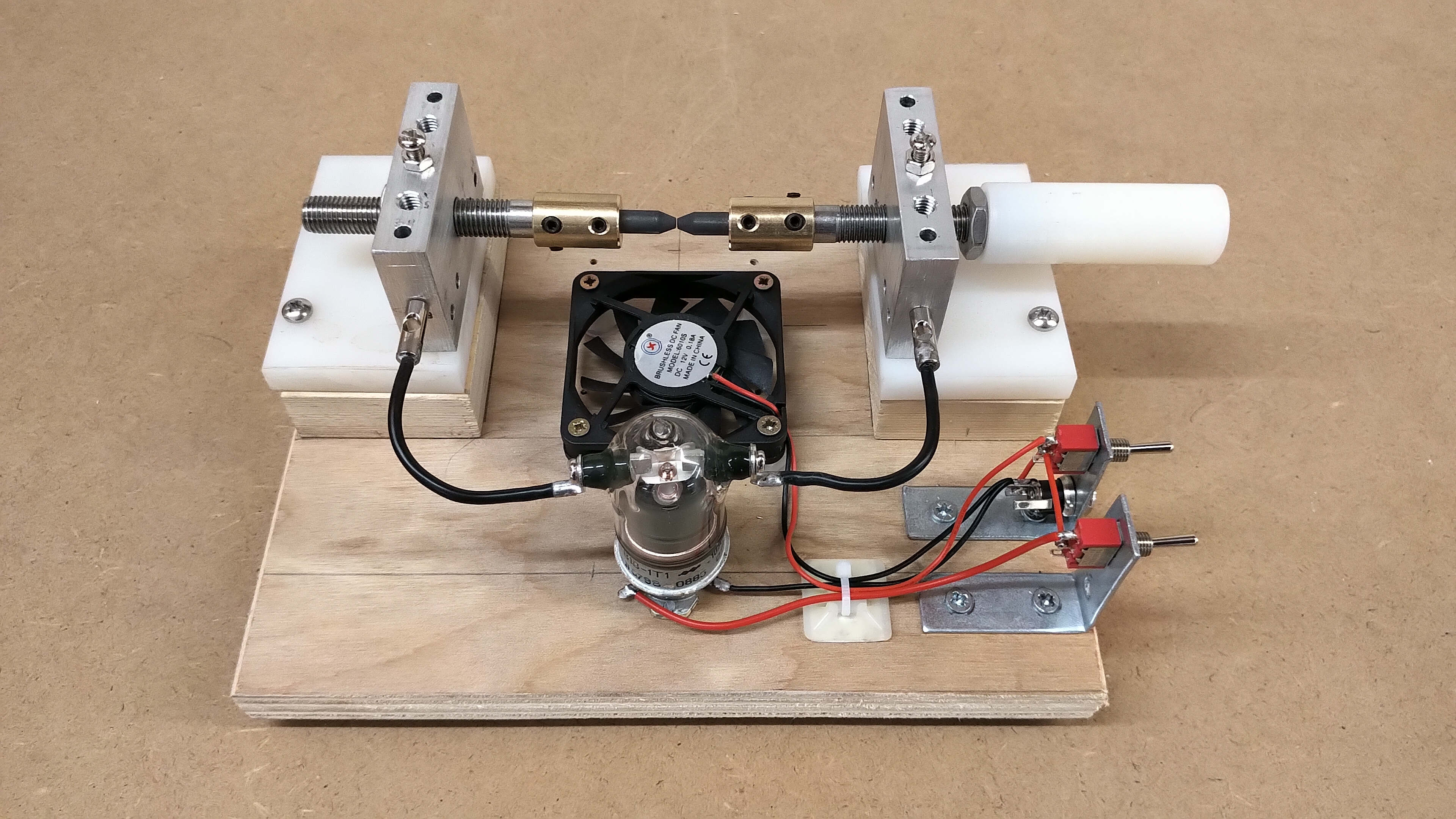
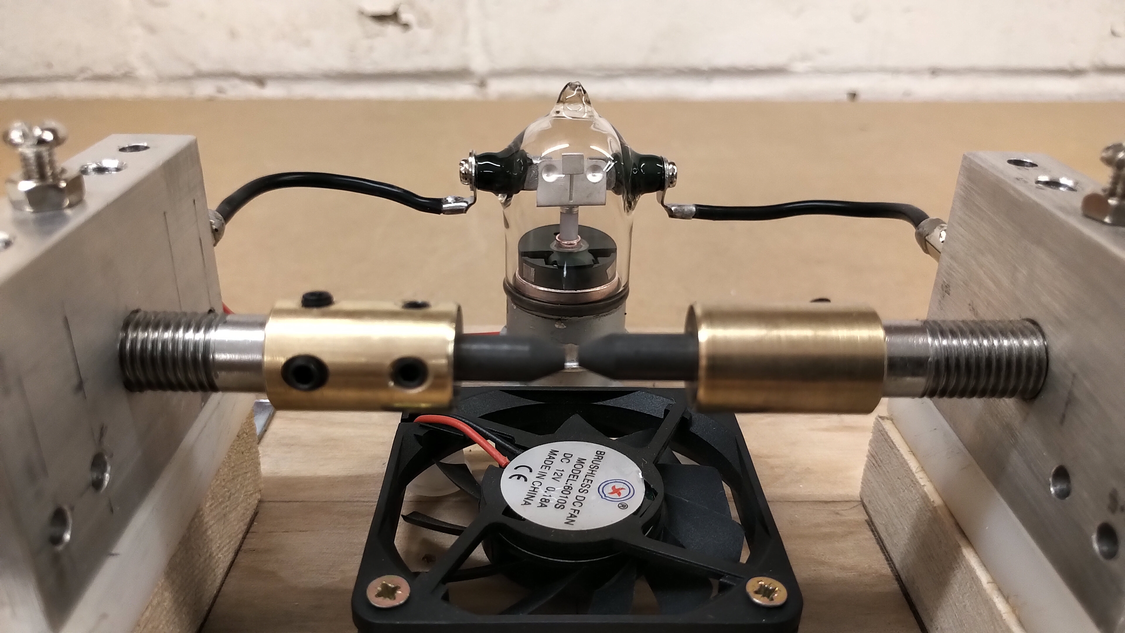
Figures 1 show the experimental apparatus and circuit, and some of the different types of measurements taken as part of the experiments.
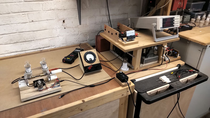
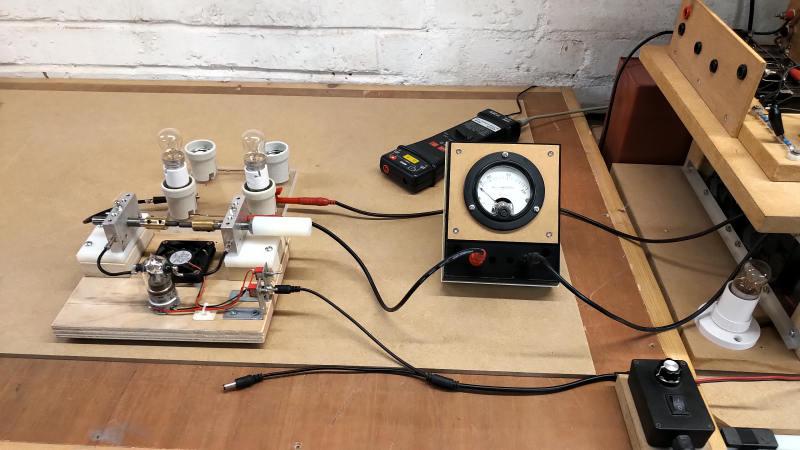
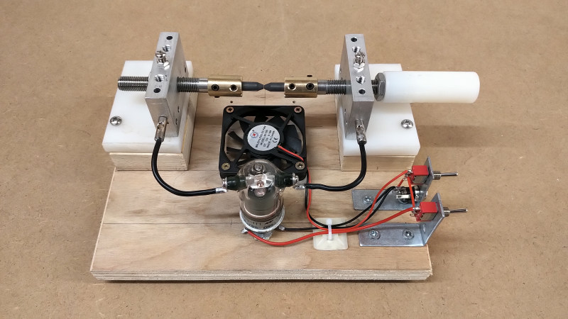
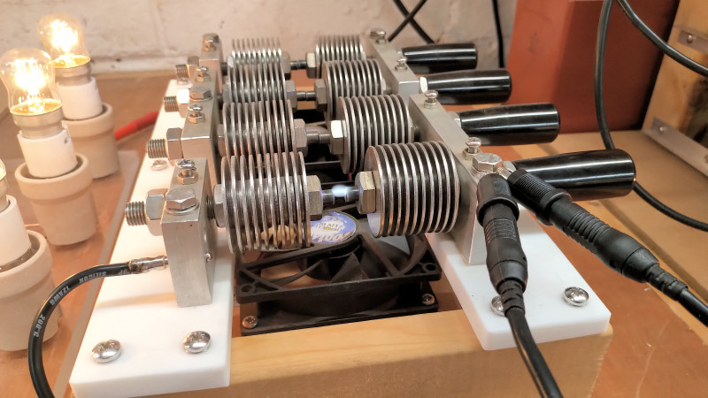
Fig. 1.1 The complete experimental setup including the HV supply and rectifier, Yokogawa power meter and rf ammeter, carbon arc spark gap (CSG), and the incandescent lamp load.
Fig. 1.2 The 200mA RF thermo-ammeter is used to monitor the rms current in the experimental circuit. Non-linear transient drive from the generator is necessary to utilise the negative resistance region of the CSG.
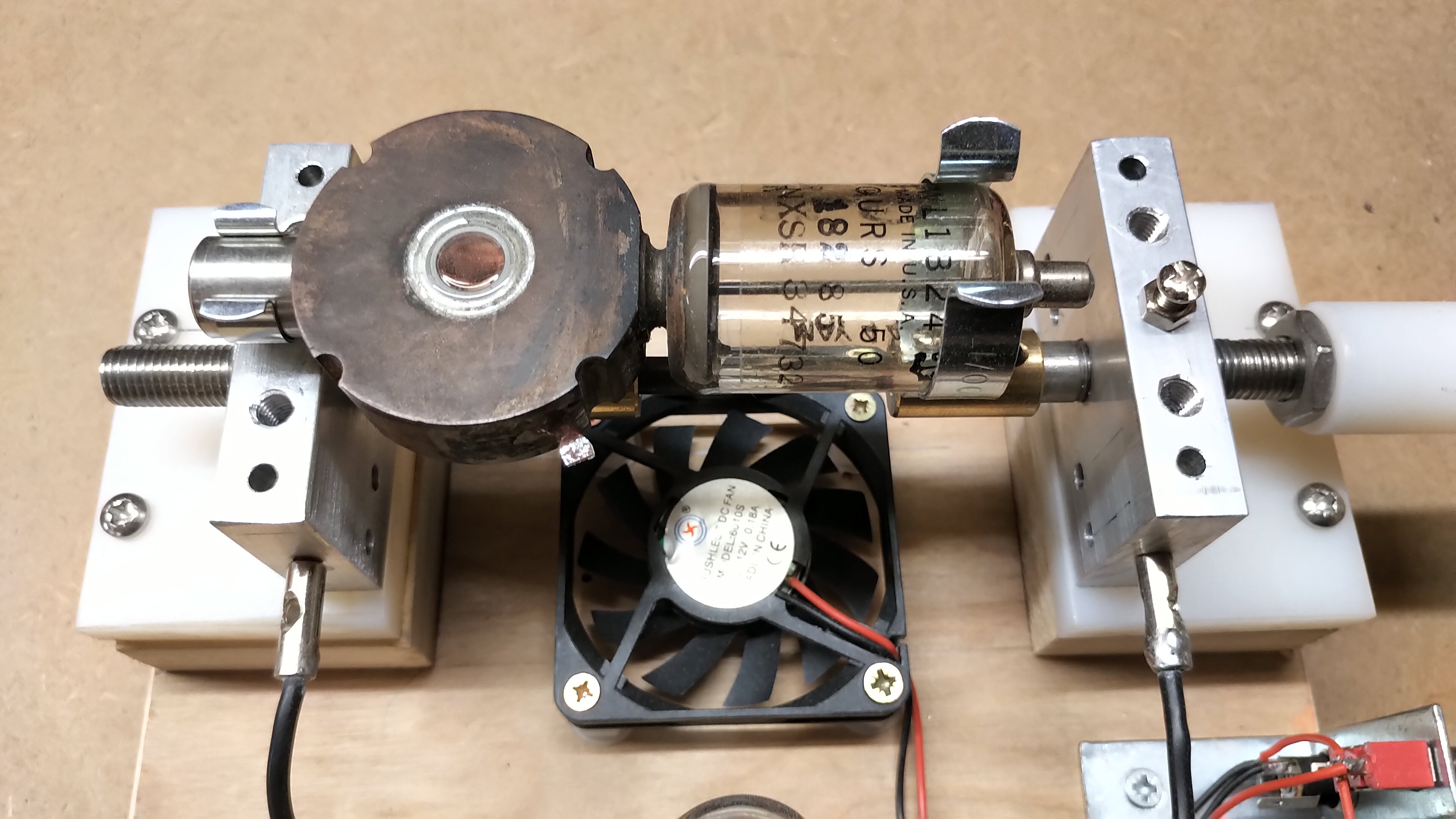
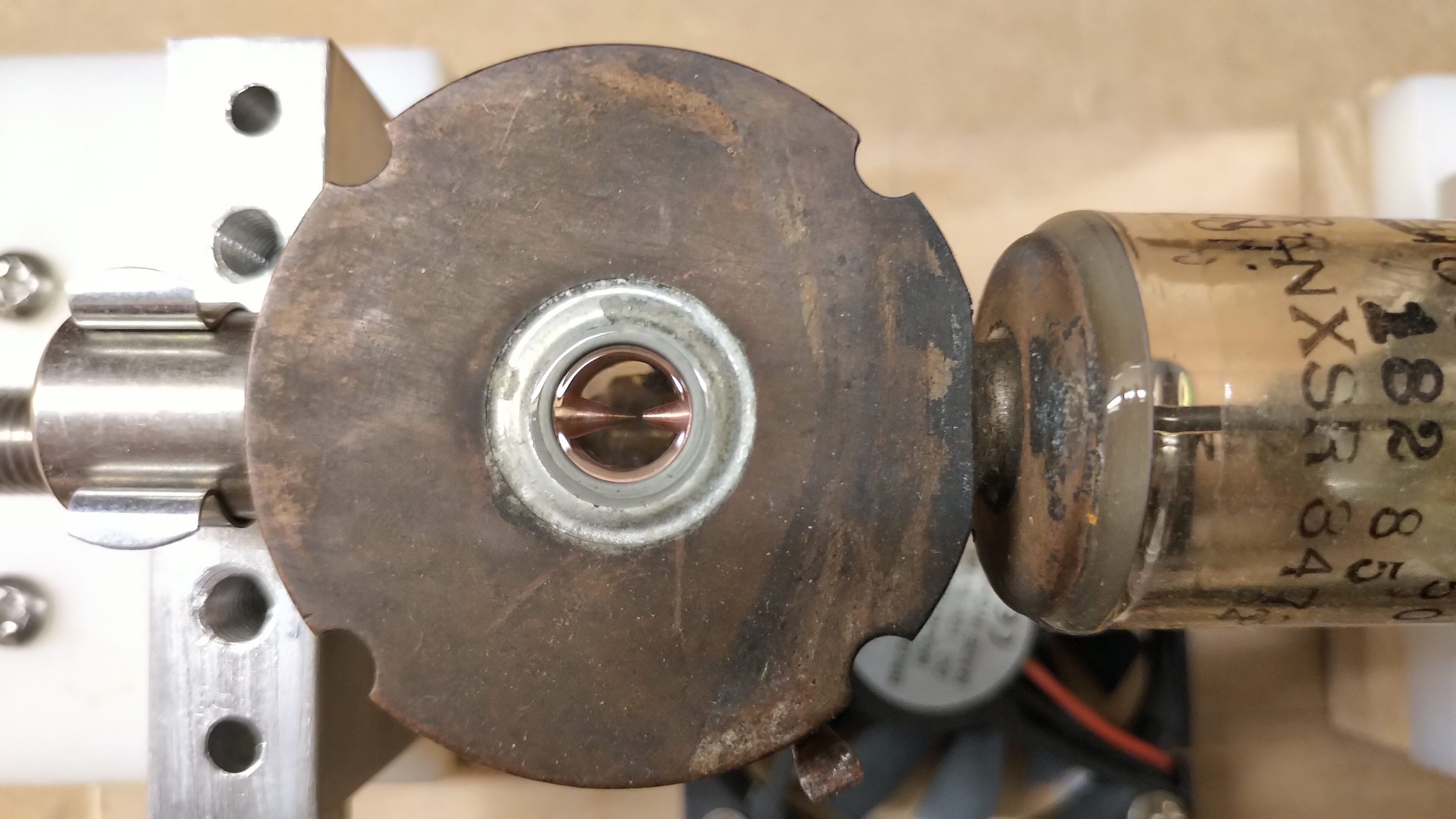
Fig. 1.3 The carbon electrode gap size can be adjusted using the nylon handle during operation. The gap is shunted by a B1B 3kV 10A vacuum relay operated from the DC 15V supply. Fan cooling of the carbon electrodes can also be used for plasma arc experiments.
Fig. 1.4 The vacuum relay provides a short-circuit path across the electrodes for circuit impedance measurements and comparison. When switched off conduction in the circuit is via the I-V characteristics of the CSG.
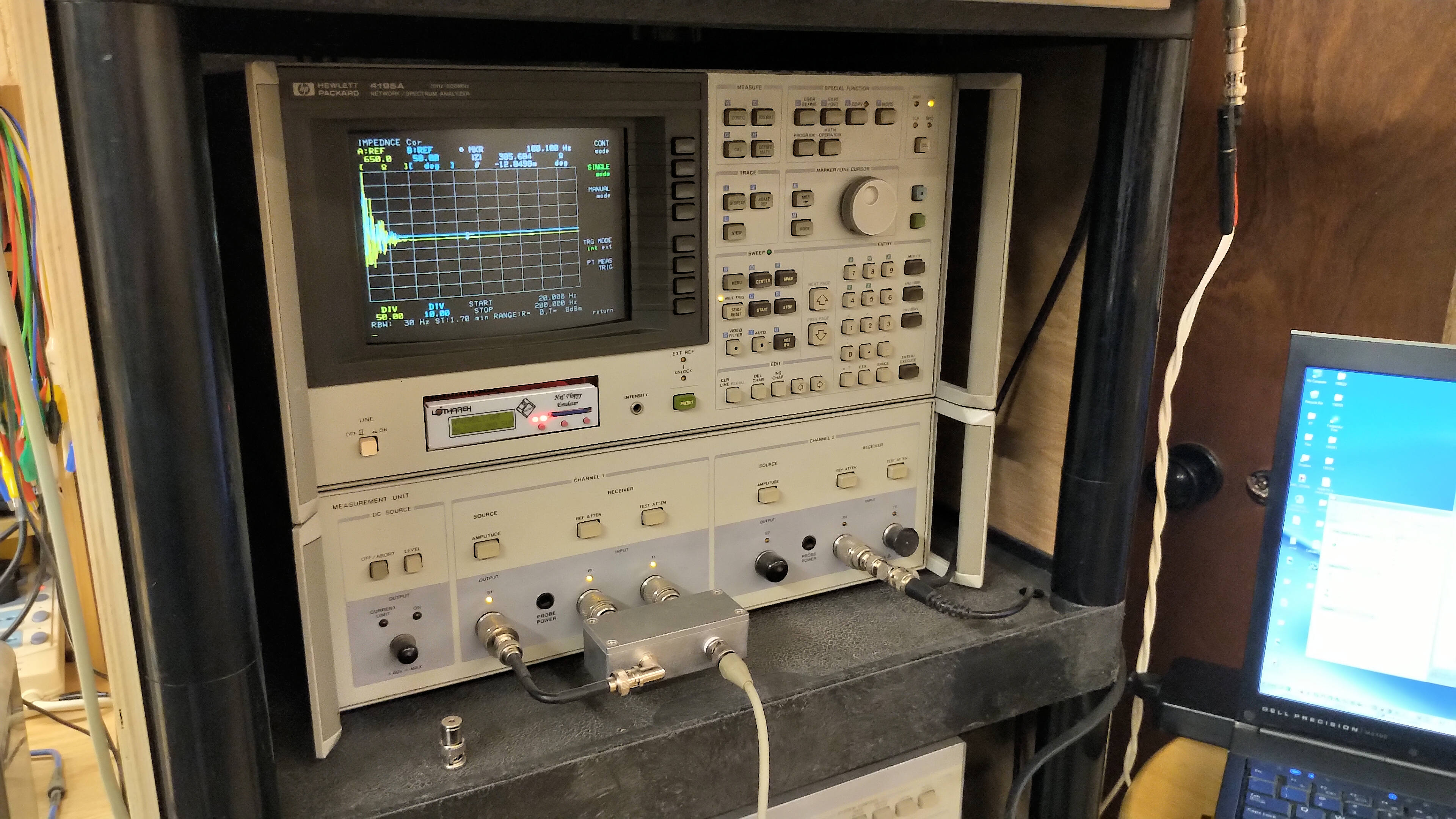
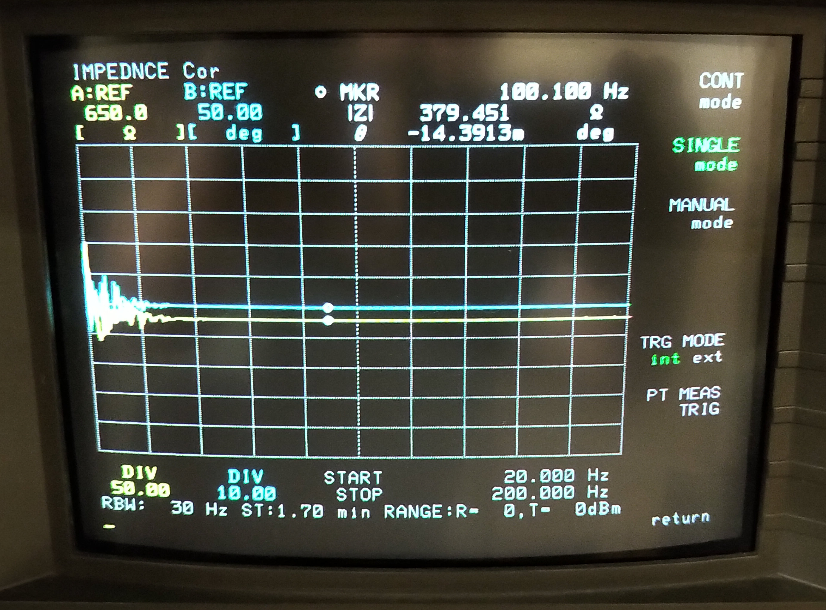
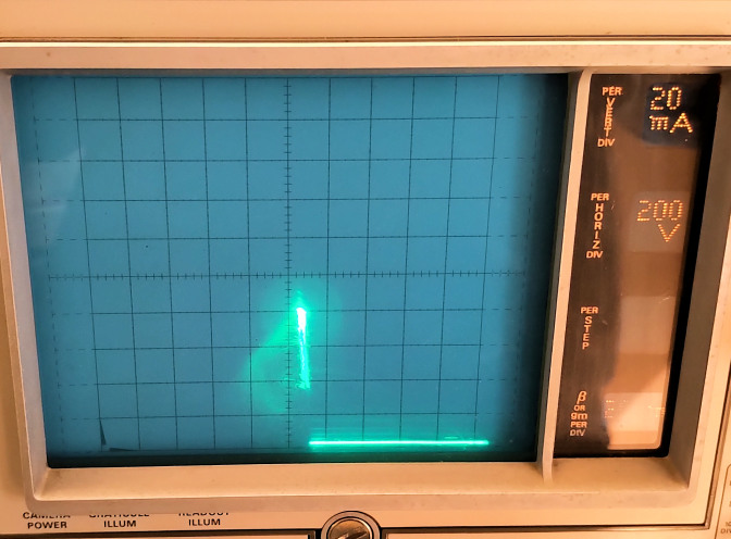
Fig. 1.5 The low frequency input impedance Z11 from the perspective of the generator, measured using the HP4195A, and showing a linear resistive impedance over the range 20-200Hz.
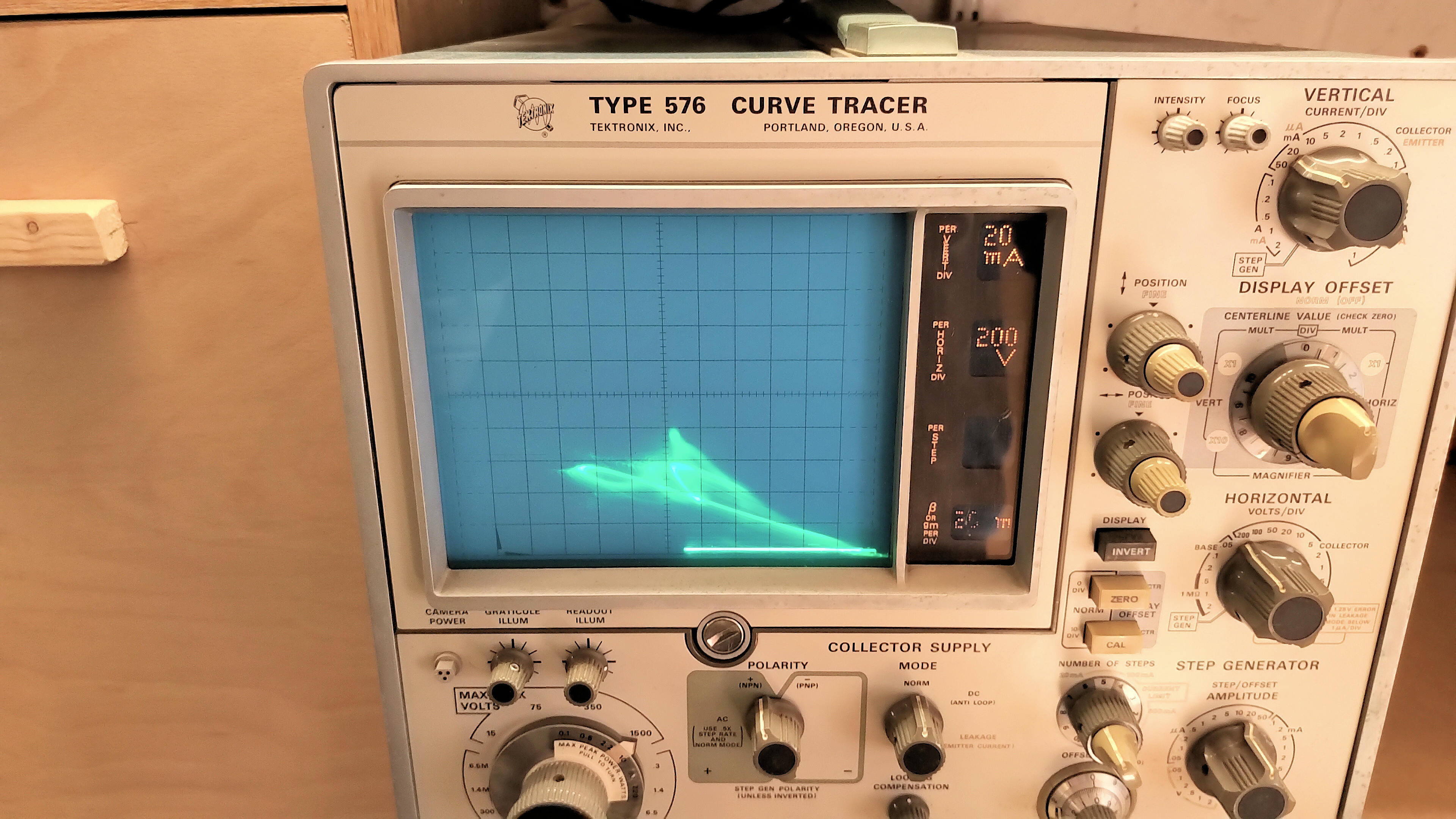
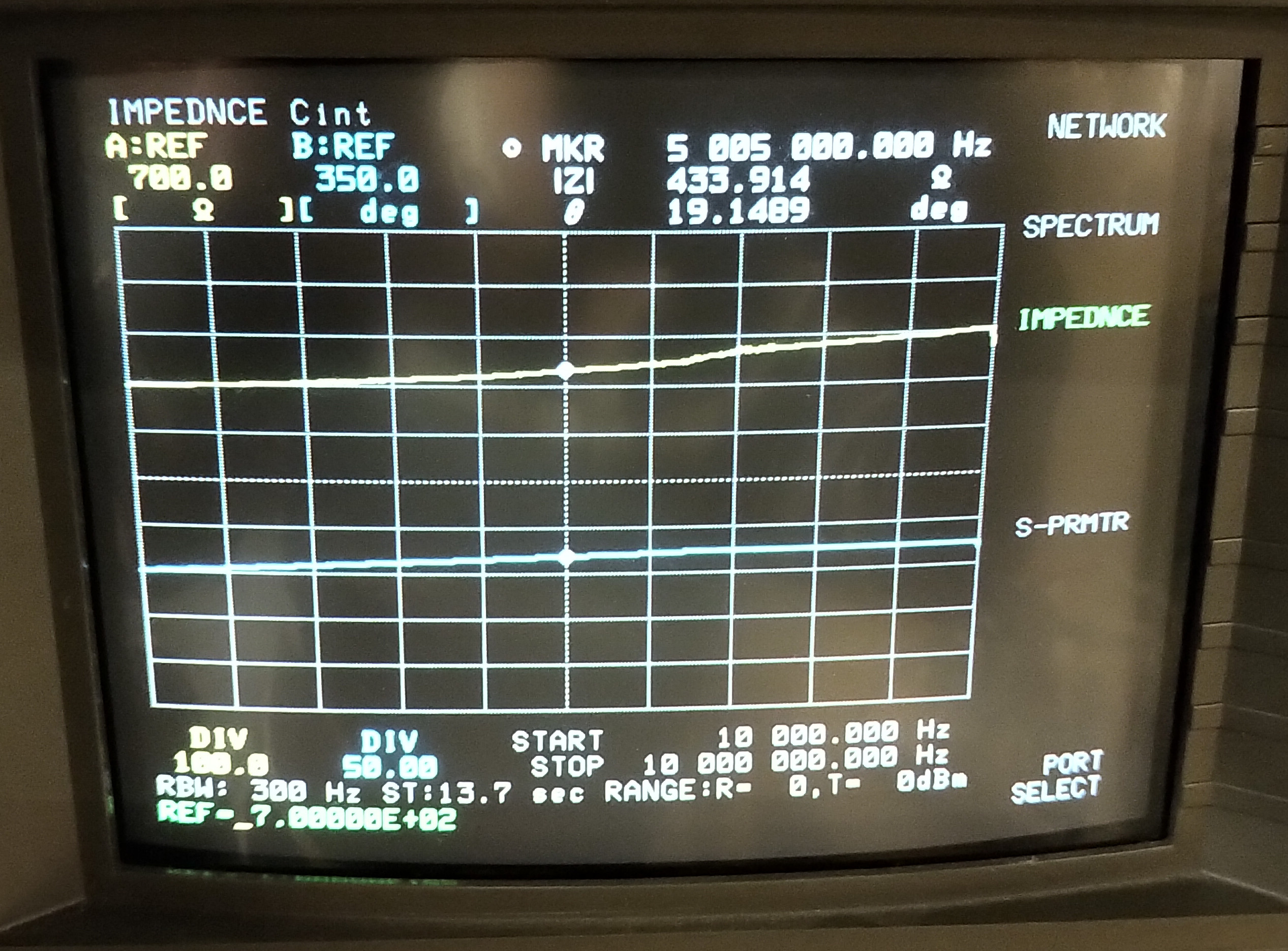
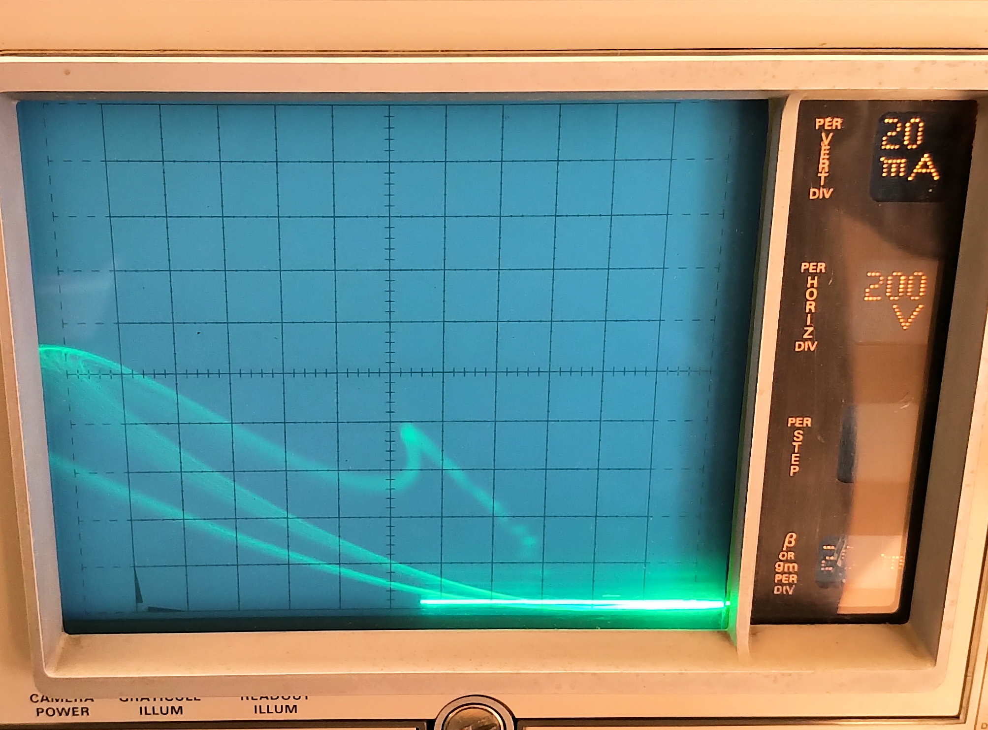
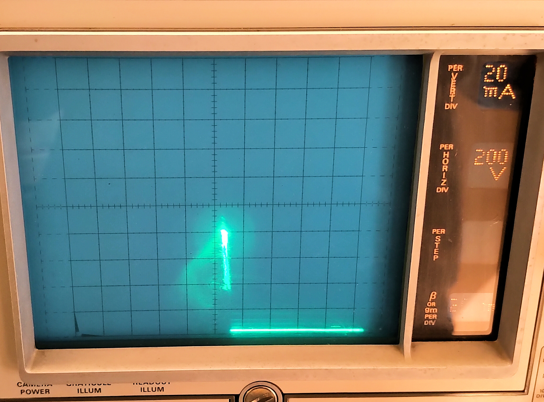
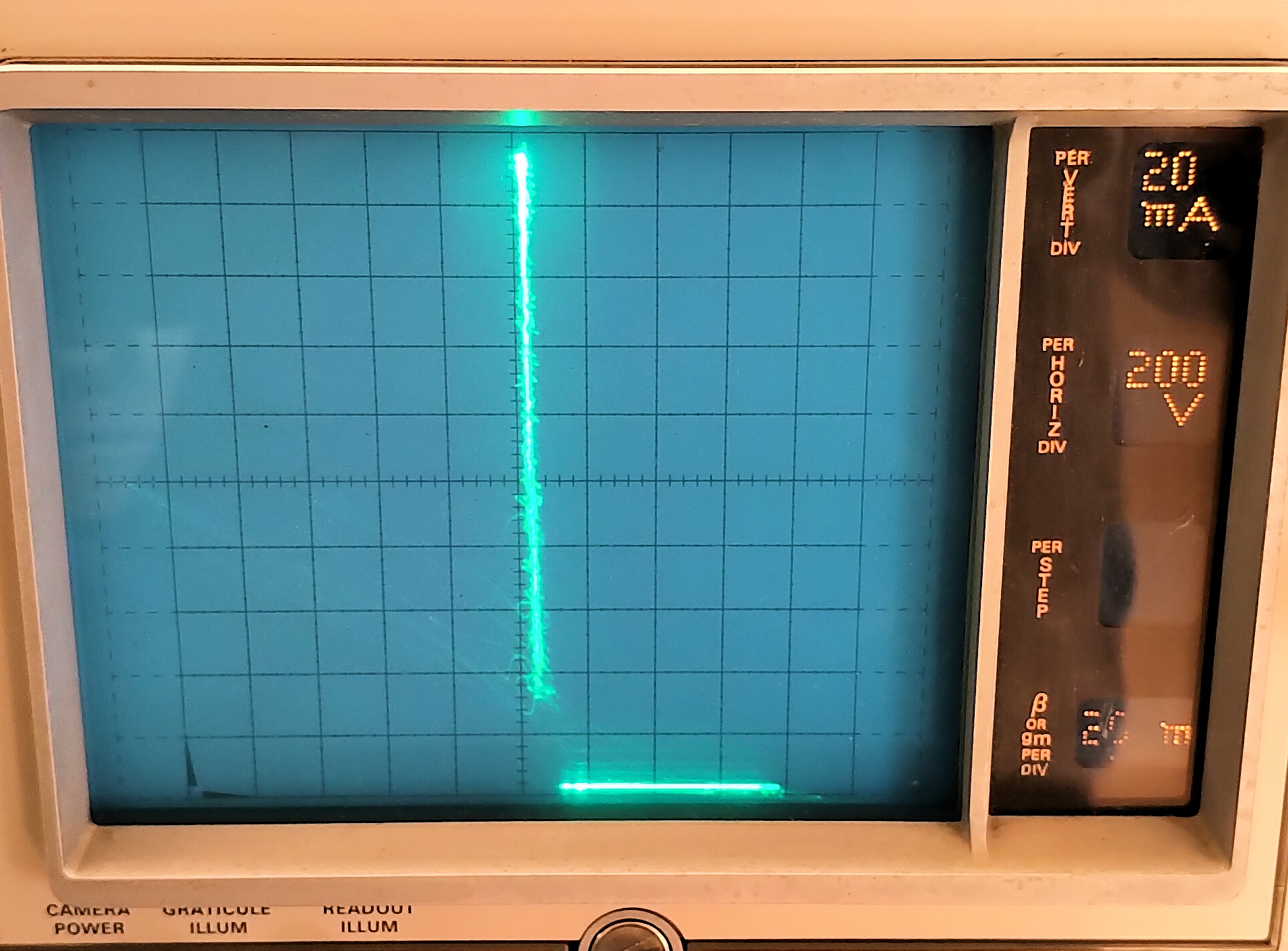
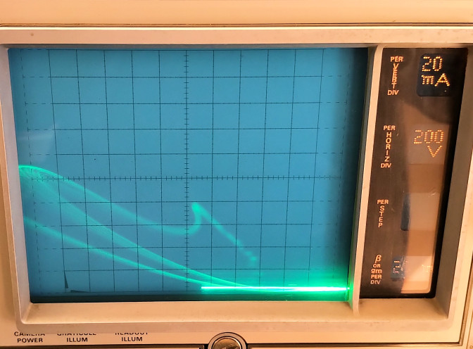
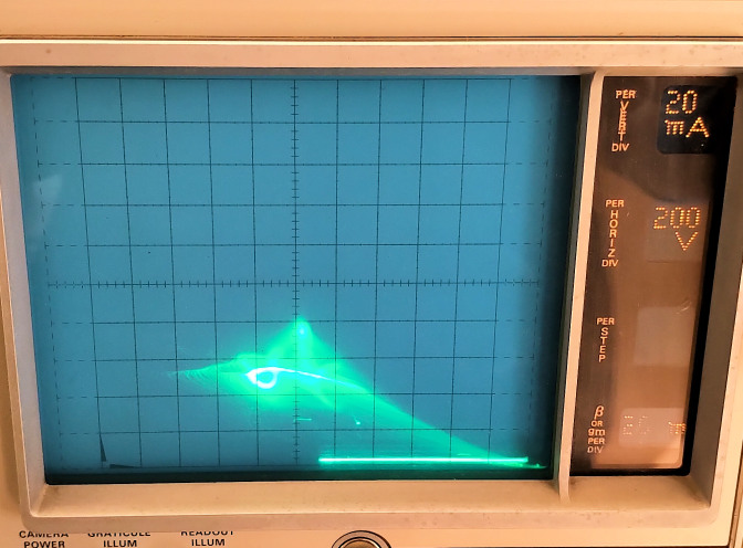
Fig. 1.6 The I-V characteristics of the CSG as measured by a Tektronix 576 curce tracer, with the measurement power limited to 10W. Here the CSG is biased into the negative resistance region prior to the onset of arc discharge.
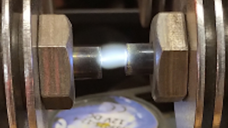
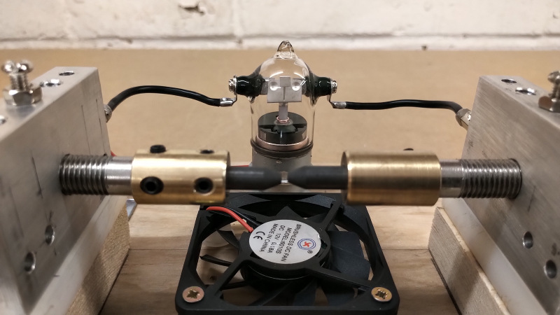
Fig. 1.7 An adaption of the experimental circuit using a single tungsten electrode spark gap, and showing the white plasma arc developed over a gap of ~ 5mm.
Fig. 1.8 A closeup view of the silent white hot plasma arc developed in the gap when switched with a non-linear transient drive. The white beam of the discharge and its surrounding halo extend over ~ 5mm electrode gap.
The generator for this experiment is a single HV transformer in the High Voltage Supply (HVS), the output is rectified and connected directly to one electrode of the CSG via an RF ammeter, (Weston 425 200mA FSD). The other electrode of the CSG is connected to a two lamp series incandescent load (2 x 25W = 50W) and then back to the other terminal of the HVS transformer. The CSG has fan assisted cooling, and is shunted in parallel by a 3kV 10A vacuum relay, which enables the CSG to be switched in and out of the circuit for impedance and load power comparisons. The fan and vacuum relay are driven by a low voltage 15V output provided again by the HVS. The input power to the HVS transformer is continuously measured using a Yokogawa WT200 Digital Power Meter.
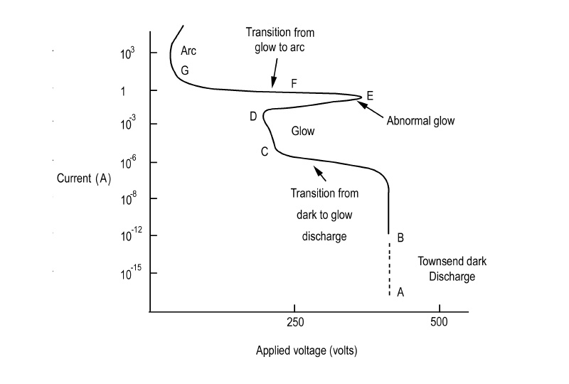
The process of ionisation in the region between two electrodes with a high electric field, is well studied in the prior art[5]. Liberated electrons within the discharge region are accelerated by the electric field between the electrodes, and in the process of moving towards the anode cause further ionisation of atoms, leading to an electron avalanche effect known as a Townsend discharge. Figure 2 below shows the typical current-voltage (I-V) characteristics for a Townsend discharge transposed from Abdelrahman et al.[6]. The negative resistance characteristics utilised in this experiment result from biasing the CSG to the correct region of this I-V curve, around the abnormal glow region between points D-E-F-G . The interesting and unusual phenomena presented in this experiment result from the reduction in circuit impedance, when the biased CSG is combined with a suitable load circuit (incandescent lamps), and driven from a non-linear transient high voltage generator at the line frequency.
Fig. 2 A typical current-voltage (I-V) characteristics for a Townsend discharge between two electrodes. The negative resistance phenomena explored in this experiment result from biasing the CSG around the abnormal glow region, between points D-E-F-G.
The following video introduces the apparatus, experiments, and phenomena associated with the negative resistance of a CSG, and demonstrates aspects of the following:
1. A qualitative observation of the discharge produced in the CSG when biased into different regions of the I-V characteristic, including open-circuit, short-circuit, abnormal glow (D-E-F), and arc discharge (G) regions.
2. Adjusting and biasing the spark gap into the abnormal glow region to utilise the negative resistance properties within the electrical circuit.
3. The change in impedance of the circuit when switched between short-circuit conduction and spark gap discharge.
4. The change in circuit current and dissipated power in the load with switched impedance, and the effect on the input power to the generator from the line supply.
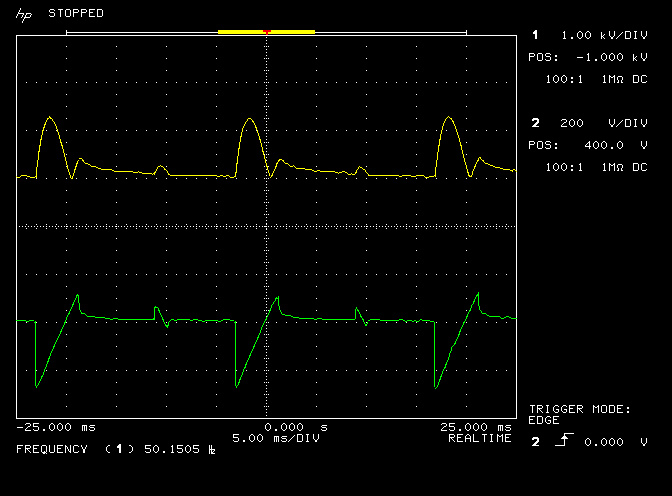
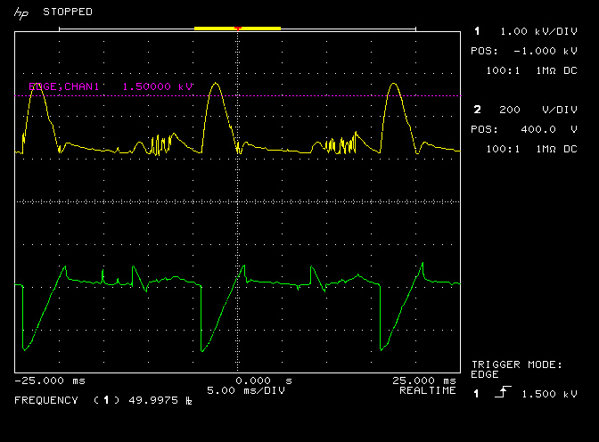
5. A comparison of adjusting and biasing the circuit when driven from a non-linear transient input, and a linear sinusoidal.
6. Measurement of the generator output using an oscilloscope both in the non-linear and sinusoidal cases, and showing the switching transients generated when the CSG is biased into the negative resistance region.
7. An experimental investigation of the I-V characteristics of the CSG using a Tektronix 576 curve tracer.
Figures 2 below show in detail some of the additional measurements made during the experiment including the overall impedance properties Z11 of the experimental circuit from the perspective of the generator, the different drive conditions applied from the generator, and the NR characteristics of the CSG measured on the Tektronix 576 I-V curve tracer.
Fig. 3.1 The low frequency input impedance Z11 for the experimental circuit with the vacuum relay on as a short-circuit across the CSG. The resistive impedance is dominated by the cold resistance of the lamp loads.
Fig. 3.2 The HF input impedance Z11 of the experiment up to 10Mc. The low frequency resistive impedance increases due to inductance of the cables in the circuit, and with no self-resonant properties in the band.
Fig. 3.3 The input to the HV transformer at the SCR output (green), and the output of the HV rectifier (yellow). The SCR creates a switched non-linear pulse drive to the experiment.
Fig. 3.4 The CSG is adjusted to utilise the NR region of the I-V characteristics. Impulse currents from discharges in the CSG are present, along with an increase in peak voltage at the HV rectifier output ~1.8kV.
Fig. 3.5 I-V characteristics of the CSG on a Tektronix 576 curve tracer. The output power of the tracer is limited to 2.2W @ 1500V. In the NR region the trace rapidly sweeps negative in a wide arc before coming back toward the centre bias point at around 80mA.
Fig. 3.6 Tracer output power limit 10W. At 1200V the transition to the NR region is reached. The transition is quicker with less magnification to the left of the screen, and a tighter and more direct path to the centre bias point.
Fig. 3.7 Tracer output power limit 50W. The loops of the NR region are just visible, and show how rapidly the onset of arc discharge occurs when the circuit current is less restricted.
Fig. 3.8 Tracer output power full 220W. The wide arcs of the negative resistance region are just visible, but the transition through this region is very rapid. The arc discharge is fully developed in region G+ (Fig. 2).
To view the large images in a new window whilst reading the explanations click on the figure numbers below:
Fig 3.1. Here we look at the low frequency small signal input impedance Z11 from the perspective of the generator, using the HP4195A network analyser. The circuit was measured and compared in two conditions, firstly with the carbon electrodes touching at the ends forming a short-circuit, and secondly with the electrodes parted and the vacuum relay activated to shunt the electrode gap with a short-circuit path through the relay. In both of these cases the impedance measured was the same in magnitude and phase and shows that above 25Hz and up to 200Hz the circuit is completely resistive at a constant 379.5Ω, and constant phase of ~ 0° (-14.4 mdeg @ 100.1Hz). Below 25Hz will also be a continuous constant resistive impedance but requires considerably reduced resolution bandwidth to remove the measurement noise observed. A reduced resolution bandwidth in this case represents a considerably increased scan time for the measurement. This measurement shows that there are no unusual impedance characteristics at the base drive line frequency, no resonant characteristics, and that the circuit appears as a constant resistive load that results almost entirely from the cold resistance of the incandescent lamp filaments, 2 x 25W in series, (in the range 175 – 200Ω each).
Fig 3.2. Shows the HF small signal input impedance Z11 from the perspective of the generator up to 10Mc, using the HP4195A network analyser. The SCR in the HV supply creates a switched output from the incoming sinusoidal line supply, (see Fig. 3.1 here for detailed input and output waveforms), which means there are many higher frequencies present at the output of the HV transformer. This constitutes a non-linear transient drive to the experimental circuit, which is the summation of many higher frequencies, and hence higher frequency characteristics of the circuit impedance contribute to the overall circuit operation, and may play a part in the observed phenomena. This is then combined with the high frequency transient switching in the spark gap itself, which adds a much wider band of available frequencies, and the all important impulse-like currents in and around the abnormal glow discharge region. We can see from this measurement that the resistive impedance rises gradually with frequency reaching ~ 434Ω @ 5Mc, and ~503Ω @ 10Mc. There are no significant features in the measured band, the circuit is not self-resonant up to 10Mc, and the overall circuit is largely resistive with a small amount of series stray inductance from the the wiring.
Fig 3.3. Shows the oscilloscope waveforms both for the input to the HV transformer at the output of the SCR (green), and the output of the HV rectifier at the input to the experimental circuit (yellow), where the circuit is set with the vacuum relay closed across the CSG. The SCR output shows how the line sinusoid is chopped into a small section, in this case part of the negative half of the cycle, providing pulses of input current to the HV transformer. The output of the HV rectifier is a voltage magnified pulse train up to ~ 2kV, and set at ~1.3kV peak for this experiment. This output level is sufficient to generate discharges in the CSG, whilst low enough to allow fine control of the I-V characteristics through electrode gap adjustment.
Fig 3.4. Here the vacuum relay has been opened and the CSG adjusted to utilise the NR region around the abnormal glow section of the I-V characteristics. The basic form of the waveforms are the same as in Fig. 3.3 with the addition of some impulse currents from discharges in the CSG, an increase in peak voltage at the output of the HV transformer ~ 1.8kV, and a slight increase in the “on” cycle of the SCR from ~ 4ms to 5ms. This corresponds to increased brightness in the lamp loads, an increased current in the experimental circuit from ~ 100mA to 125mA, and an increase in the power drawn from the line supply ~ 50W to 80+ W. The bias adjustment of the SCR remains the same as for the condition in Fig 3.3, yet clearly by operating the CSG around the abnormal glow region of its characteristics more power is drawn in through the line supply, reflecting a reduction in impedance in the experimental circuit below that of the normal short-circuit impedance at the CSG electrodes or through the vacuum relay. When the experimental circuit is biased at this point the region between the carbon electrodes is mostly dark and visibly discharge free, with the occasional momentary white flash as a discharge occurs across the electrodes when point G (Fig. 2) is reached.
Fig 3.5. Shows the I-V characteristics of the CSG as measured on a Tektronix 576 curve tracer. The advantage of a purely analog curve tracer like this is that negative resistance can be easily visualised through the unusual movement of the beam spot, which through the thickness and luminescence of the trace shows the speed of movement, and through the path of the spot often in arcs and loops, the unusual characteristics of NR regions and transitions. In this test the output power of the tracer is limited to 2.2W at maximum voltage bias of 1500V. With the current in the CSG restricted with a high series resistance (300kΩ) arc discharge does not occur, and the electrical characteristics can be explored prior to the arc discharge at point G. Here the voltage across the electrodes has been increased to the full 1500V output. At the transition voltage the gap enters the NR region and the trace rapidly sweeps negative in a wide arc before coming back toward the centre bias point at around 80mA of current, and still prior to arc discharge. The low luminescence of the arc shows the very rapid transition through this region, and the length of the arc right across to the far left of the screen, shows how the NR effect magnifies the voltage across the high series resistance in the test circuit.
Fig 3.6. Here the output power of the tracer is set to 10W limit, with a series resistance of 65kΩ. At 1200V output the transition to the NR region is reached, but here the transition is even quicker which less voltage magnification to the left of the screen, and a tighter and more direct path to the same centre bias point of around 80mA of current prior to arc discharge. Without current limiting in the circuit the transition through the NR region is very rapid, which makes biasing a circuit to maintain characteristics at this point both tricky and mostly unstable, as could be seen in the video experiment. It is better to establish a circuit that oscillates around the NR region and hence utilising its unusual properties in a more stable manner, then trying to bias statically to one individual bias point within the NR region.
Fig 3.7. Here the output power of the tracer is set to 50W limit, with a series resistance of 14kΩ. At 1100V output the CSG transitions rapidly to arc discharge, indicated by the bright region at about 50V 80mA. The loops of the negative resistance region are just visible, and show now how rapidly the onset of arc discharge occurs when the circuit current is less restricted.
Fig 3.8. Shows the full development of the arc discharge curve at the maximum power output limit of 220W, with a series resistance of 3kΩ. The wide arcs of the negative resistance region are just visible, but the transition through this region is very rapid and in this case utilisation of that region would become very difficult as the characteristics of the CSG are dominated by the arc discharge. With the arc discharge fully developed in region G+ (Fig. 2) it is interesting to note that the impedance presented by the circuit is now higher then the short circuit case, the lamps are dimmer, and a lower current is drawn from the line supply. The impedance of the circuit can be further lowered by shorting the CSG with the vacuum relay, which increases the brilliance of the lamps to the CSG short-circuit case. The impedance of the circuit can be further lowered from the CSG short-circuit case by opening the vacuum relay, and adjusting the electrode spacing to bias the characteristics into the negative resistance region. At this point the lowest impedance of the circuit is presented to the HV supply, drawing the maximum current and hence power from the line supply.
The negative resistance characteristics in the discharge region, and the ability to adjust and utilise this region, appear to be strongly influenced by two material factors in the circuit:
1. The electrode material used for this experiment is carbon which shows a negative resistance region over an adjustable range. It is repeatedly possible, as demonstrated in the video, to adjust and maintain the CSG into the abnormal glow region of the curve and observe unsual phenomena in the circuit. When the carbon electrodes were replaced with tungsten electrodes it became very difficult to adjust the CSG into a region where the NR characteristics could be maintained. Adjustment to the correct bias could only be accomplished momentarily before reverting to the arc discharge region, or the open circuit condition. This suggests that the bias region for the abnormal glow is much narrower and hence much more difficult to select in a metal such as tungsten. As such the properties of carbon are identified as a more suitable material for the I-V characteristics that lend themselves to the utilisation of negative resistance within non-linear electrical systems.
2. The gaseous medium within the discharge region between the electrodes. In this first part on this topic, and for simplicity in the video, experiments were demonstrated with air in the discharge region, but considerably better results have been obtained when the electrodes are in a vacuum region or inert gas inside a glass tube. Two mechanisms have been tested to demonstrate this, the first a vacuum relay where the gap between the electrodes could be adjusted by applying a dc current to the relay’s exciter coil, and secondly a 1B24 TR cell, a cold cathode tube RF spark gap, where the internal gap can be adjusted by an external screw. A TR cell is a gas discharge tube which is used typically as an electronic switch, or as in the case of the 1B24, to protect the sensitive receiver of a radar system from damage by the strong transmit pulse. This method in radar is now long obsolete, the 1B24 being used in, and just after, the second world war. The tube used here has a manufacture date of May 1944 printed on the glass.
Figures 3 below shows the arrangement of the 1B24 TR cell which was used in experiments to enhance the phenomena presented in this post.
Fig. 4.1 The vintage 1B24 TR cell, (manufactured in 1944), is mounted in place of the cardon electrode. The rest of the circuit remains the same.
Fig. 4.2 The TR cell is held in place using metal spring clips. The lower small clip forms the cathode connection, and the upper anode is connected by a fly lead mounted directly to the aluminimum mount (not shown).
Fig. 4.3 The waveguide mounting section of the 1B24 contains the adjustable copper spark gap, visible through the glass window section in the centre of the mount. The spark gap region and chamber are filled with an inert gas to improve discharge quenching.
Fig. 4.4 The inner copper electrode on the lower side of the spark gap can be adjusted by the flat-head screw in the base of the waveguide mount. Adjusting this during operation allows biasing in to the NR region of the I-V characteristics.
In the case of the vacuum relay it was found that a very small gap could be controlled by adjusting the dc current in the relay exciter coil. At a certain level of bias the contact would start to switch between closed and a very tiny gap, both exploiting the negative resistance in I-V characteristics, whilst introducing another transient switching source in the circuit. In this case the overall resistive impedance in the circuit fell considerably lower than that experienced with the correctly biased CSG. The current in the secondary circuit went up as far as 200mA, the lamps where illuminated with a very high brilliance, and the input power drawn from the generator increased considerably to reflect this rapid decrease in circuit impedance. This bias method and utilisation of NR whilst intensified, was difficult to maintain, and would quickly destabilise to normal circuit impedance. However, this experiment shows that the utilisation of NR properties is strongly dependent on the degree of transient switching and hence non-linearity in the circuit, and combined with a clean discharge region, in this case the vacuum relay contact gap, considerable intensification of the phenomena is possible.
Summary of the results and conclusions so far
The phenomena observed in this experiment and demonstrated in the video, and combined with additional supporting measurements, appears to result from a reduction in circuit impedance below that of a short-circuit condition, when the CSG is adjusted into the negative resistance region surrounding the abnormal glow section of the I-V characteristic. When adjusted to this region, and combined with a non-linear transient drive from the generator, the overall impedance of the circuit drops, and the current rises as more power is drawn from the generator. In this experimental case the increase in brilliance of the incandescent lamps results from additional power drawn from the generator, over and above that drawn when the CSG is directly short-circuited by the vacuum relay. From this we can ascertain that the negative resistance region of the CSG reduces the overall circuit impedance presented to the generator in non-linear transient cases. In this experiment there is no evidence of additional energy being drawn into the circuit from any source other than the generator, and all changes in energy can be accounted for by measurement of that supplied into the HV supply, and that dissipated in the load.
In comparison, when the HV supply was driven using a linear sinusoidal from a variac, rather than a non-linear switched SCR controller, the phenomenon could not be adjusted, observed, or measured in the same experiment, and the impedance of the circuit under all conditions using the CSG is greater than the short-circuit of the vacuum relay, or carbon electrodes. From this it is clear that to utilise the unusual properties of negative resistance they must be combined with a non-linear impetus, which also suggests a process that may be related to underlying displacement events. It is always in the presence of a non-linear condition that the mechanism of displacement can be engaged or observable within the electrical properties. It appears to surface in non-linear scenarios where the boundaries of the dielectric and magnetic fields of induction would lead to a discontinuous condition in the electrical properties of the circuit. It is conjectured that displacement appears to “act” in order to rebalance this discontinuous condition and restore dynamic equilibrium between the induction fields within the circuit.
With regard to the phenomenon observed in this experiment, it is conjectured that the apparent reduction in circuit impedance below that of a short-circuit primarily results from a coherent inter-action between the dielectric and magnetic fields of induction. The analogy is drawn to both the superconducting state in metals at low temperature[7,8], and also to ballistic electron transport in a high mobility electron gas[9], also at low temperature. In the case of the superconducting state two electrons became weakly bound together through exchange of a lattice phonon. In so doing they form Cooper pairs where the coherent phonon exchange extends across the entire material on a macroscopic scale. This coherent phonon exchange, and subsequent binding together of Cooper pairs, leads to a band-gap opening in the conduction band of the material, and hence electron-pairs can traverse the dimension of the material without scattering in this band. In this way conduction of a current via electron movement through the superconducting material has zero resistance, and is considered to be coherent.
In the second case of ballistic electron transport, the electronic energy band structure of the semiconductor is so arranged to provide a quantum well, narrower than the phonon wave number, at the fermi level within the well. This confines electrons to a 2D sheet in the well, reducing scattering and increasing the mean free path. Further confinement laterally leads to a 1D wire where the scattering with the lattice is further reduced and the mean free path of an electron becomes longer than the injection contacts at either end of material. In this case, and at low temperature, electrons can travel ballistically from one terminal to the other (e.g. in a quantum wire channel). The ballistic conduction reduces the resistance between the contacts below that normally expected for the diffusive condition, since the scattering with the lattice has been reduced to a point where the electron path between the contacts can be considered as coherent.
In both of these analogies reduction in impedance of the transmission medium is considered the result of a coherent conduction process. In the experiment reported here I conjecture that the reduction in impedance results from the coherent inter-action of the dielectric and magnetic fields of induction, where that coherent configuration is brought about by a displacement event. The displacement event is in itself revealed through the non-linear drive to the experiment, and “mixed” through the negative resistance properties of the CSG. The final product of the displacement event through the negative resistance characteristics, is to re-balance the electrical dynamics of the circuit by coherently aligning the dielectric and magnetic fields of induction yielding a reduced circuit impedance. This conjecture, based on the results so far, requires considerable further work to establish its scope of validity, and would also ideally benefit from a suitable mathematical treatment, when such a form of mathematics is available to describe the properties and processes under exploration.
For further exploration and discussion on the results and phenomenon from this experiment please see the Energetic Forum[10].
In the experiments of Chernetsky[1], and others[3,4], the SGD occurred when the carbon electrodes were adjusted, presumably, into the negative resistance region of their I-V characteristics. The generator for this experiment was a switched fly-back transformer, (transient driven), between 25-100kc, and the secondary circuit incorporated a tank capacitor charged from a half-wave rectified output from the secondary coil of the fly-back. The load was formed with incandescent lamps in series with a carbon electrode gap, and connected in parallel with the secondary tank capacitor. When the carbon arc gap was properly adjusted in the experimental circuit, the current supplied to the fly-back primary was seen to fall, whilst the lamp load was illuminated with greater brilliance, and no discharge arcs where visible between the carbon electrodes. The additional energy in the circuit to maintain the brilliance of the lamps was attributed to energy drawn into the circuit from the Aether and the circuit is claimed to be OU in performance.
The experimental circuit explored in this preliminary investigation of negative resistance is different to that of Chernetsky and others for the following main reasons:
1. It operates at the line frequency of 50Hz, much lower than the 25-100kc of the fly-back transformer.
2. It does not include a tank capacitor in the secondary, which made lead to additional resonant circuit and/or magnification phenomena in the secondary, and possibly cavity effects and hence longitudinal modes formed between the secondary of the fly-back and the external circuit.
3. A bridge rectifier is utilised instead of half-wave rectification of the secondary output.
Differences 1 and 2 may certainly be significant to the overall result and performance of the circuit. On this basis it is not possible yet to support or refute the OU claims for this circuit. Certainly the non-linear negative resistance phenomena explored in this experiment does not result in an OU condition. In the next part of this experimental sequence the same CSG is used in a circuit equivalent to that presented by Chernetsky and others, and its overall performance measured in detail.
Update
A recent replication of this experiment by Bierbaumer[11] demonstrates that in a very similar experimental arrangement, the increased light intensity observed in the lamps, and the measured additional power drawn from the supply, is most likely to occur due to a slight preferential phase shift between the voltage and current waveforms in the SCR envelope. In this experiment the phase shift appears to be brought about by impulse noise generated by discharges in the carbon spark gap, which effects the triggering conditions of the SCR in the most basic trigger circuit. It is subsequently demonstrated that improvement of the SCR triggering circuit, to make it less susceptible to impulse noise generated by the spark gap, suppresses the observed phenomena of increased lamp intensity and additional consumed power.
Bierbaumer also uses an alternative approach to the replication of the negative resistance I-V characteristics, using a digital and analogue oscilloscope in X-Y mode, and series connected carbon-silicon spark gaps. In this experiment he demonstrates anomalously high “shoot-through” or impulse currents, which are considerably larger than expected from the measured circuit impedance, and appear to occur right at the point where the spark gap transitions between the abnormal glow region at region E (ref. Fig. 2 at the top of the post), through the transition from glow to arc at region F, and finally into the arc at G. The result of this demonstration appears to show that despite the considerable current limiting in the discharge circuit from a low inductance, high resistance load, high intensity impulse currents and the associated magnetic induction field can be generated around the negative resistance region of the carbon-silicon spark gaps.
In my own experiments I have measured similar large anomalous impulse currents in the I-V characteristics when the previously mentioned B1B vacuum relay, or the 1B24 cold cathode RF spark gap, were connected in parallel with the existing carbon-arc gap, and adjusted to the critical region on the I-V characteristrics at E-F-G. The result was much larger than expected impulse currents that could not be accounted for through SCR waveform phase relationship changes, or the measured impedance of the experimental circuit. The generation of excess impulse currents is an area that requires further investigation and careful quantitative measurement to establish if it is directly the result of negative resistance characteristics, or part of other non-linear phenomena that can arise from displacement of electric power.
1. Chernetsky, A., About physical nature of biological energy phenomenons and its modeling, All-Union Correspondence Polytechnical Institute, Moscow, 1989.
2. Whittaker, E., A History of the theories of aether and electricity, Longman, Green and Co., 1910.
4. Dawson, D. Notes on the Impulse discharge, Post #2765, Energetic Forum, 2020.
5. Little, P., Electron-emission – Gas discharges, Handbuch der Physik XXI, Springer-Verlag, 1956.
6. Abdelrahman, M. & El-Khabeary, H., Study of Three Different Types of Plasma Ion Sources, Plasma Science and Technology, Vol.11, No. 5, Oct. 2009.
7. Bardeen J. & Cooper, L. & Schrieffer, J., Theory of Superconductivity, Physical Review, Vol. 108, pg. 1175, 1957.
8. Marsh, A. & Williams, D. & Ahmed, H., Supercurrent transport through a high-mobility two-dimensional electron gas, Vol. 50, No. 11, Physical Review B (Rapid Communications), September 1994.
9. Marsh, A., Superconducting contacts and Supercurrent Flow in a GaAs/AlGaAs Heterojunction, Ph.D. Thesis, Cambridge University, July 1995.
10. Forum Members, Eric Dollard Official Forum -> Eric Dollard, Post #2807 onwards, Energetic Forum, 2020.
11. Bierbaumer, W., Negative Resistance and the Self Generating Discharge – Experimental Replication, YouTube, 2021.