The flat, spiral, or pancake coil, applied to the transmission of electric energy was presented in a patent by Tesla^[1] in 1900, subsequently investigated by Dollard et al.^[2], Mackay et al.^[3], and no doubt by others. The design, implementation, and measurement of a flat coil is presented in the following sequence of posts. This coil has then been used in a range of experiments including single wire effects, wireless transmission of power, and investigations into the properties of displacement and transference of electric power. These experiments, and there results so far, will be reported in a subsequent sequence of posts.

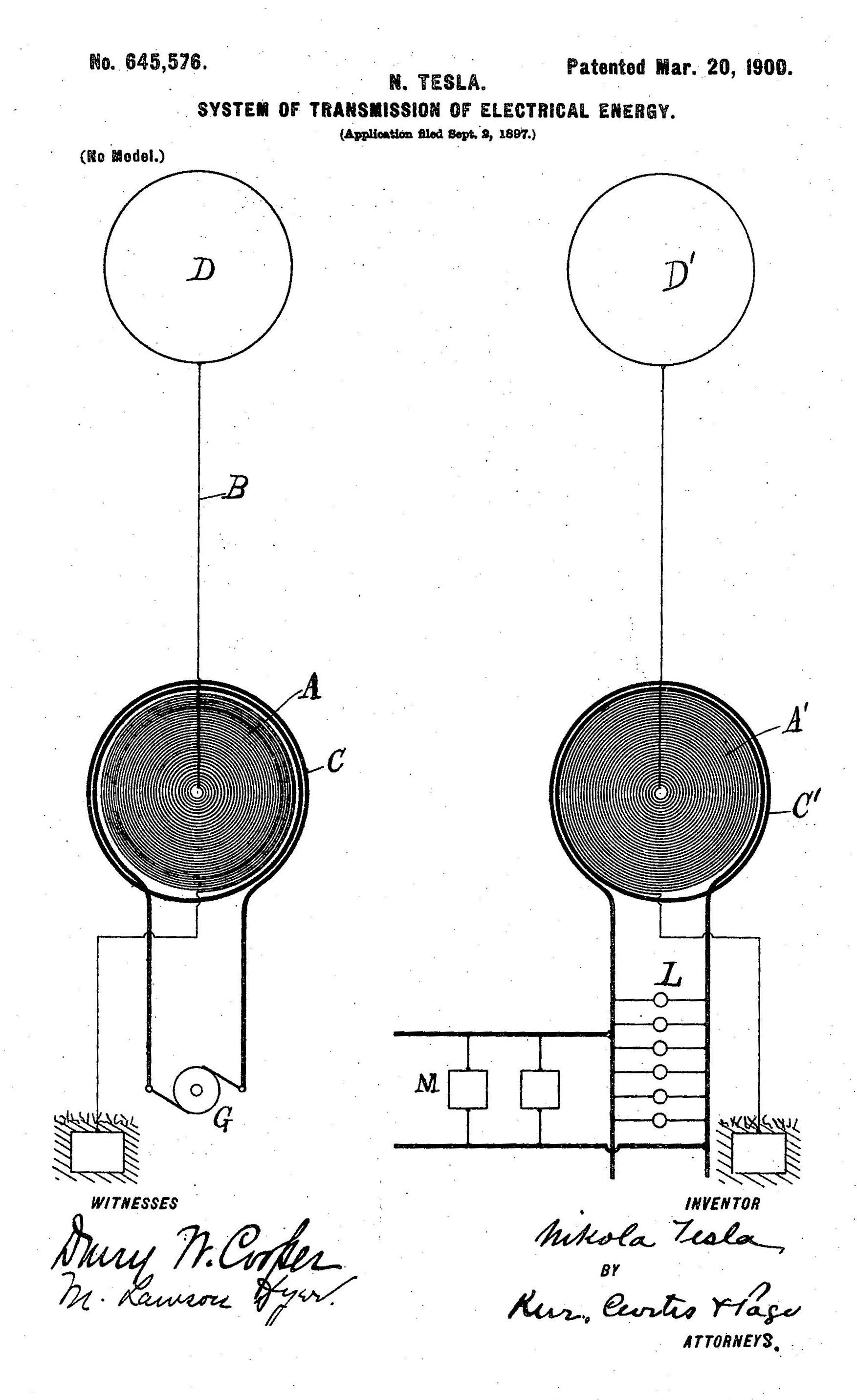
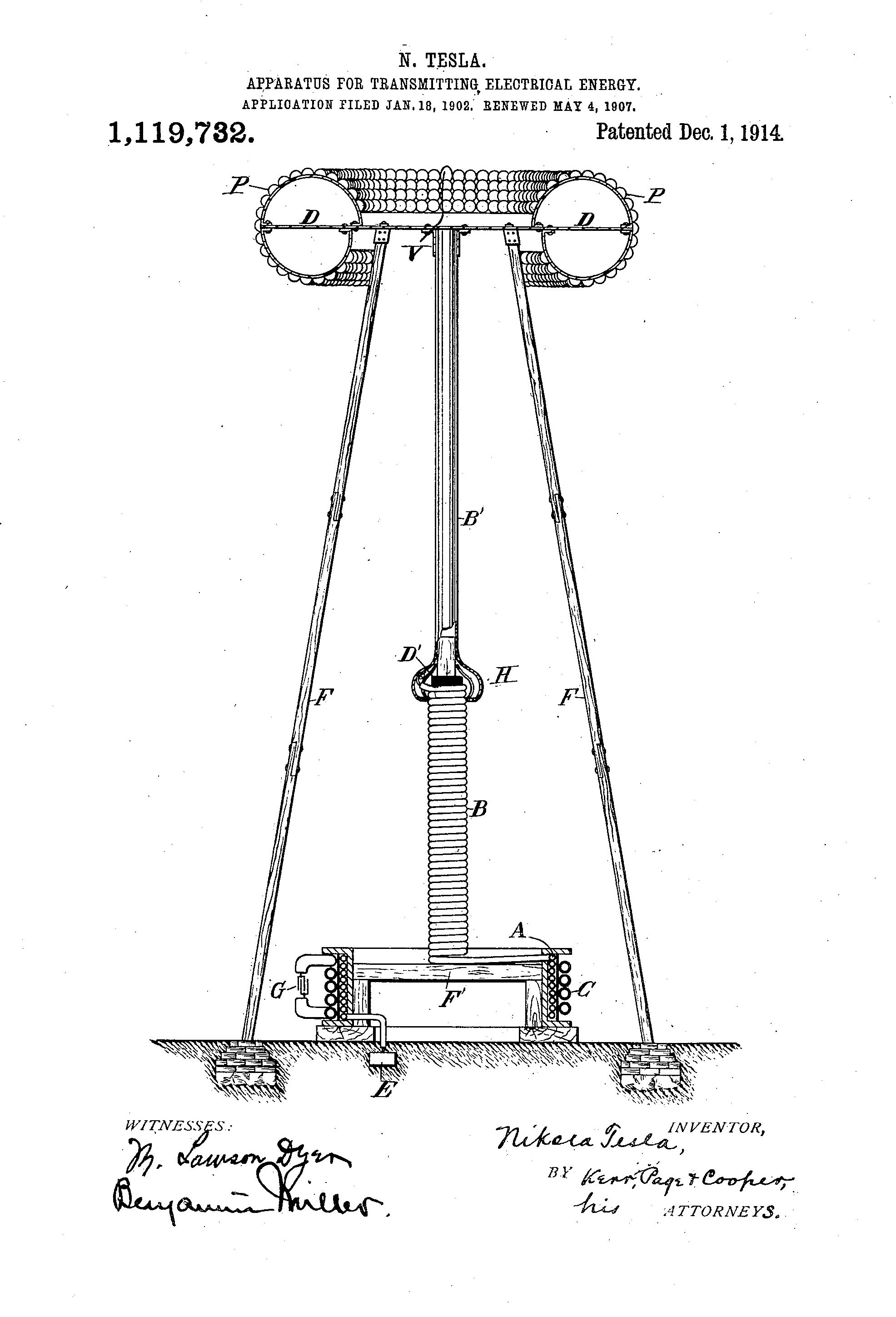
Tesla’s original design of the coil is shown in Fig. 1. Designing a flat coil empirically from scratch starts with choosing the required fundamental resonant frequency of the secondary coil. For the purposes of the intended experiments large voltage magnification is not required, and hence the flat coil comprises only Tesla’s secondary coil (λ/4) as a continuous spiral. If additional voltage magnification were required then Tesla’s extra coil^[4] (λ/2) could also be added at the top-end or central-end of the coil to make a complete tuned coil (3λ/4 or nλ/4 where n is an odd positive integer). The outer turns of the secondary coil are more closely coupled by induction to the primary coil by virtue of their closer proximity to the primary. The secondary coil, (with or without the extra coil), and in combination with the top-load or termination, accumulates energy induced from the primary and forms a resonant cavity at the designed frequency.

The properties of this resonant cavity are critical to the correct formation of the Longitudinal Magneto Dielectric (LMD) wave (standing-wave) in the coil, which may also be conjectured to be a significant pre-condition for the generation of a displacement event. The properties of the resonant cavity thus formed in a coupled free resonator, and their relationship to the displacement of electric power, will be considered in more detail in Part 2, and further at the experimental stage.

It is important to note that experiments that may include the radiation of electromagnetic energy need to comply with international radio regulation and standards, and so the fundamental operating resonant frequency of the secondary coil is to be set in the 160m amateur radio band (UK standard) in the range 1.810 – 2.000 MHz. As per Tesla’s original design, the coil is to be primarily used in a quarter-wave (λ/4) mode where the top-end or central-end of the coil is a high impedance (in this case open-circuit or connected to a top-load), and the bottom-end or outer-end of the coil is connected to a low impedance (ground, load, or other impedance lowering receptacle).

In this mode the fundamental resonant frequency of the secondary coil is firstly determined by the wire length combined with coil geometry, dimensions, and materials, all which lead to an inductive element in parallel with a capacitive element, or in electrical terms a parallel self-resonant circuit. This will set the free self-resonant frequency at which a 180^o phase change will occur in the impedance of the coil. In an ideal parallel resonant circuit this would also be the frequency at which the impedance reaches a maximum. In the practical (non-ideal) case the impedance maximum does not correspond to the frequency of phase change, but is rather reduced due to a range of factors, including:

1. The inter-winding mutual capacitance.

2. The internal series resistance of the coil.

3. Additional capacitive and other circuit loading directly to either end of the secondary coil.

4. The geometry, dimensions, materials and proximity of other conductive/insulating mediums.

5. Conducting extensions to the central and/or outer ends of the secondary coil e.g. adding an additional length of wire to either end of the coil, or a conductive ground plane.

6. The resonant frequency of other closely coupled coils e.g. the primary coil.

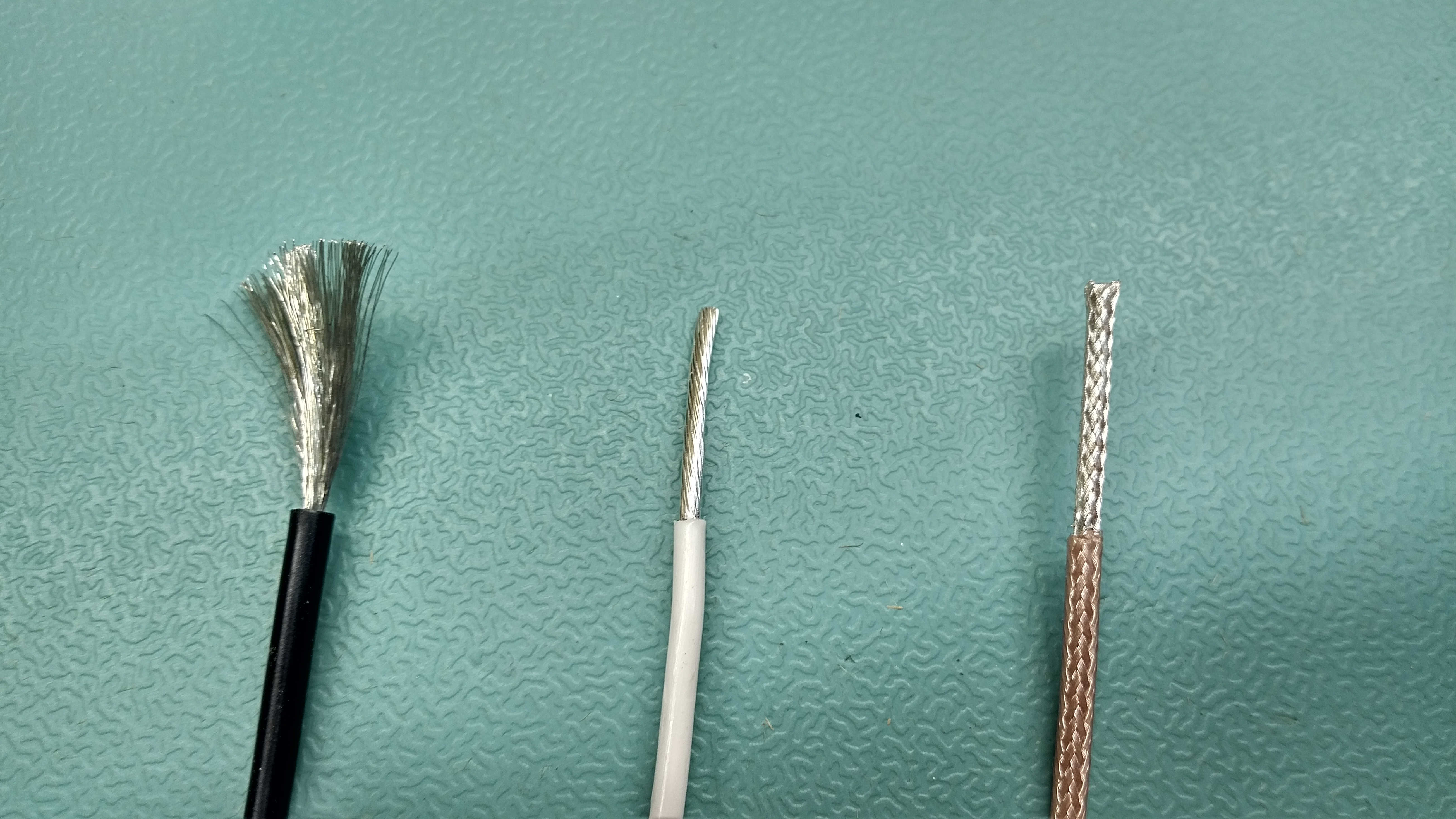
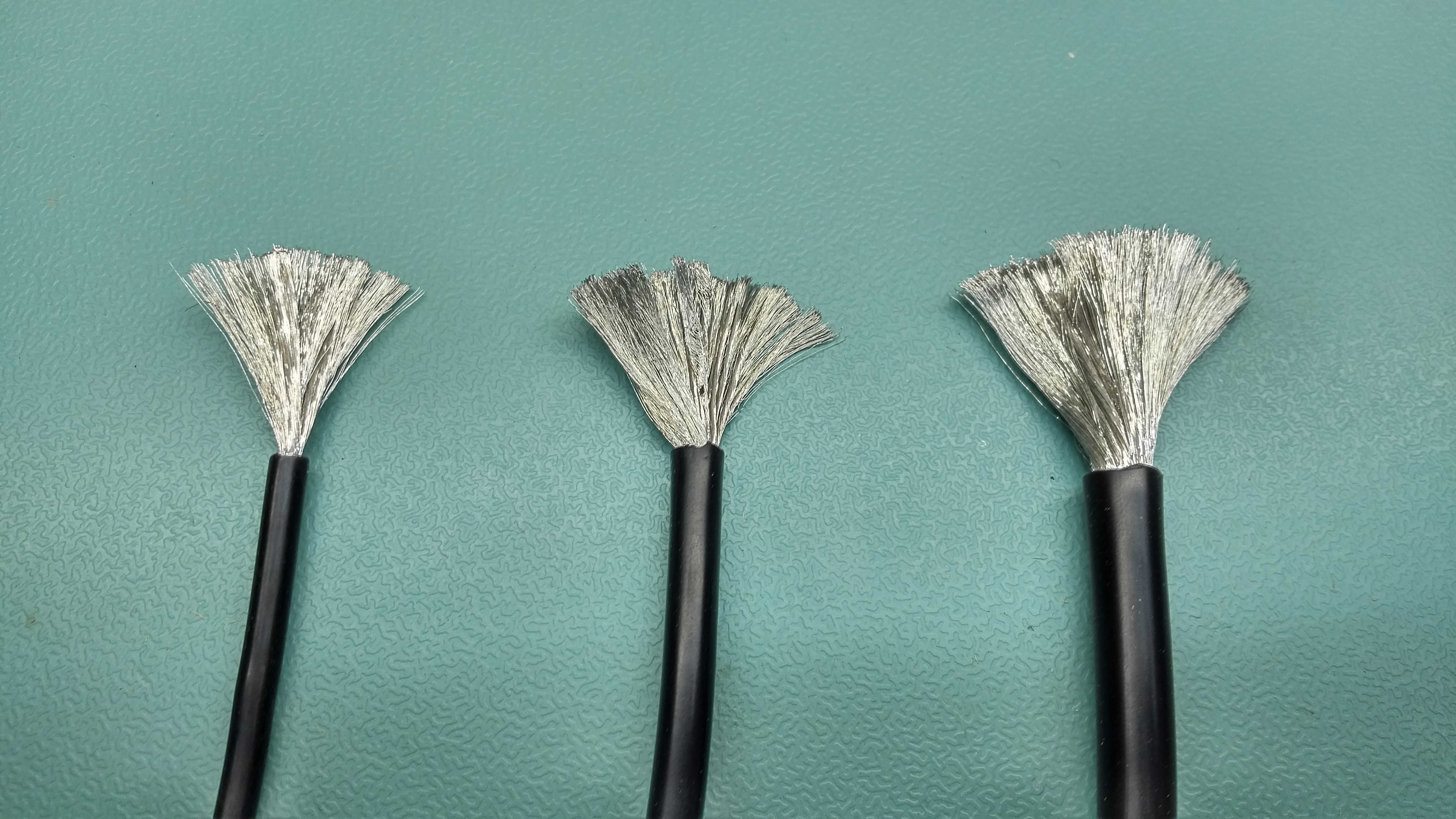
7. The wire type used for the secondary e.g. magnet wire, insulated multi-stranded, stranded coaxial sheath etc.

According to the purpose of the experiments to be undertaken using this coil, that is, the exploration of displacement and transference of electric power, the coil geometry will be designed to optimise inter-winding capacitance (coupling). Inter-winding capacitance has been suggested to make a significant contribution^[2,3] in the formation of the Longitudinal Magneto Dielectric (LMD) wave in the coil.

With this in mind the geometry of the coil is arranged with two inter-leaved layers of the coil where the number and spacing of the wire turns is arranged in order to maximise the inter-winding capacitive network, whilst keeping the fundamental resonant frequency within the required band. Arrangement of this network is by empirical methods and should ensure that the mutual inter-winding capacitance is not too high, and hence presenting too much of a capacitive load on the coil and reducing the Q, and also not too low and leading to deterioration of the required LMD wave. In other words, the magnetic field of induction and the electric field of induction must be as closely and mutually balanced in the coil as possible. This will be further considered in part 2 as an important pre-condition for the generation of a displacement event.

When the final coil(s) are incorporated into each experimental arrangement fine-tuning of the operating frequency is to be primarily affected by adjustment of the primary coil variable capacitance, and via an adjustable wire extension at the central end of the secondary coil e.g. using a short length of wire,  whip antenna, or telescopic aerial. In a parallel resonant circuit, and when the internal series resistance of the coil is significant, the minimum current at resonance occurs at a frequency lower than that expected from the ideal resonant case^[5]. In our coil design this series resistance is significant (changing with wire type and geometry) and so also contributes to a reduction in frequency of the parallel resonant impedance maximum.

It is also intended that the resonant frequency of the primary circuit will be used to tune the overall frequency characteristics of the complete coil. This will make it possible to optimise the performance of the coil in a wide range of different experimental conditions including being driven by different types of electric generators (driving the primary coil), as well as attached to a range of different loads (driven from the secondary coil). Adjustment of the resonant frequency of the primary coil causes a corresponding change in the resonant frequency of the secondary coil, and most especially when the fundamental resonant frequency is close for the two coils. The primary coil is intended to be loaded with a variable capacitance in the range 100pF – 1500pF which is suitable for tuning the coil within the desired frequency band, and additionally at frequencies above and below this band.

The accurate prediction by calculation of the self-resonant frequency of a coil is a research topic in itself, and has received considerable investigation, modelling, and experimentation over the years. A detailed theoretical and modelled study of helical resonators has been presented by Corum et al.^[6]. An experimental investigation into the properties of coil resonators has been presented by Knight^[7], and who introduces a system of analysis and testing that is closely related to the work being undertaken here. In the coil design being considered the required fundamental resonant frequency of the coil is to be established by empirical methods, and combined with fine adjustment when the coil is to be constructed and operated.

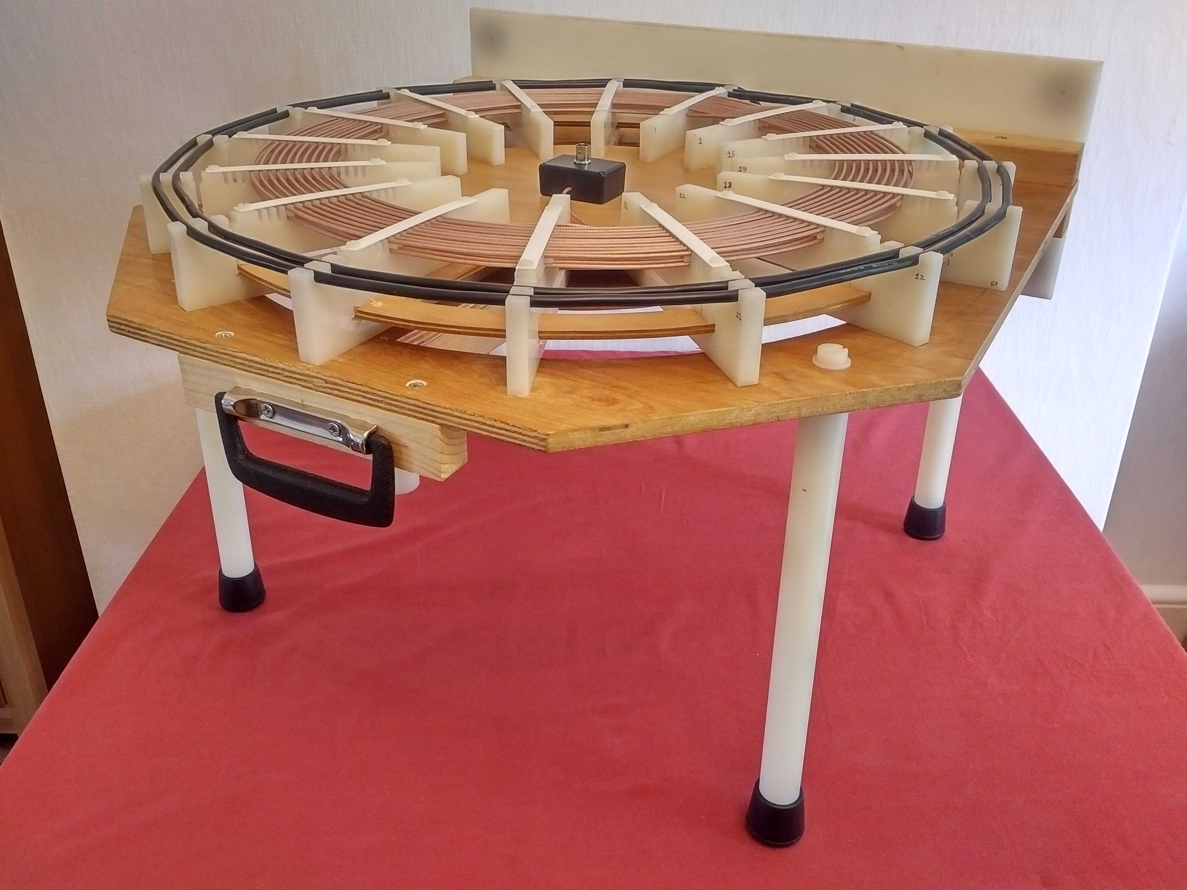
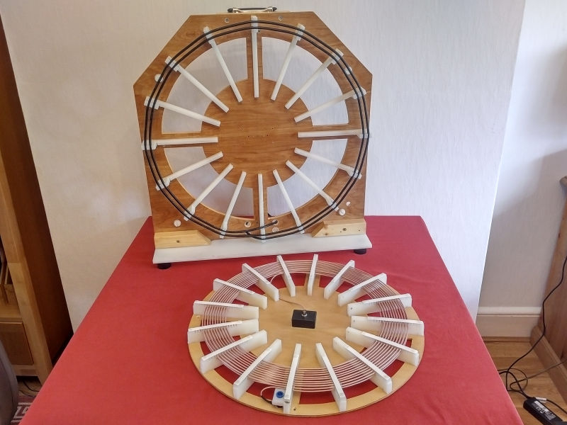
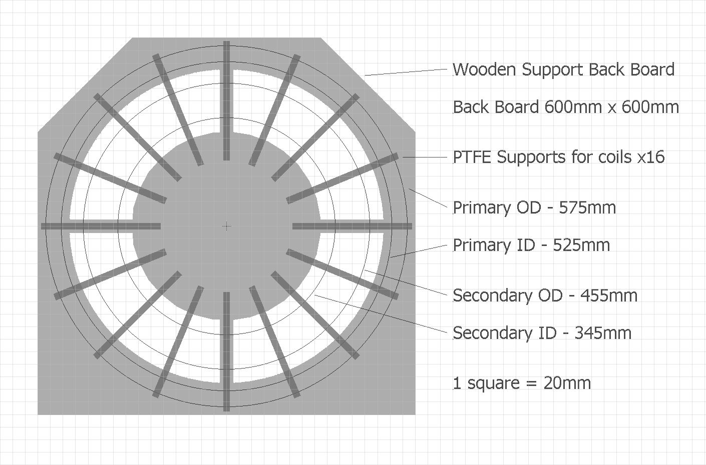
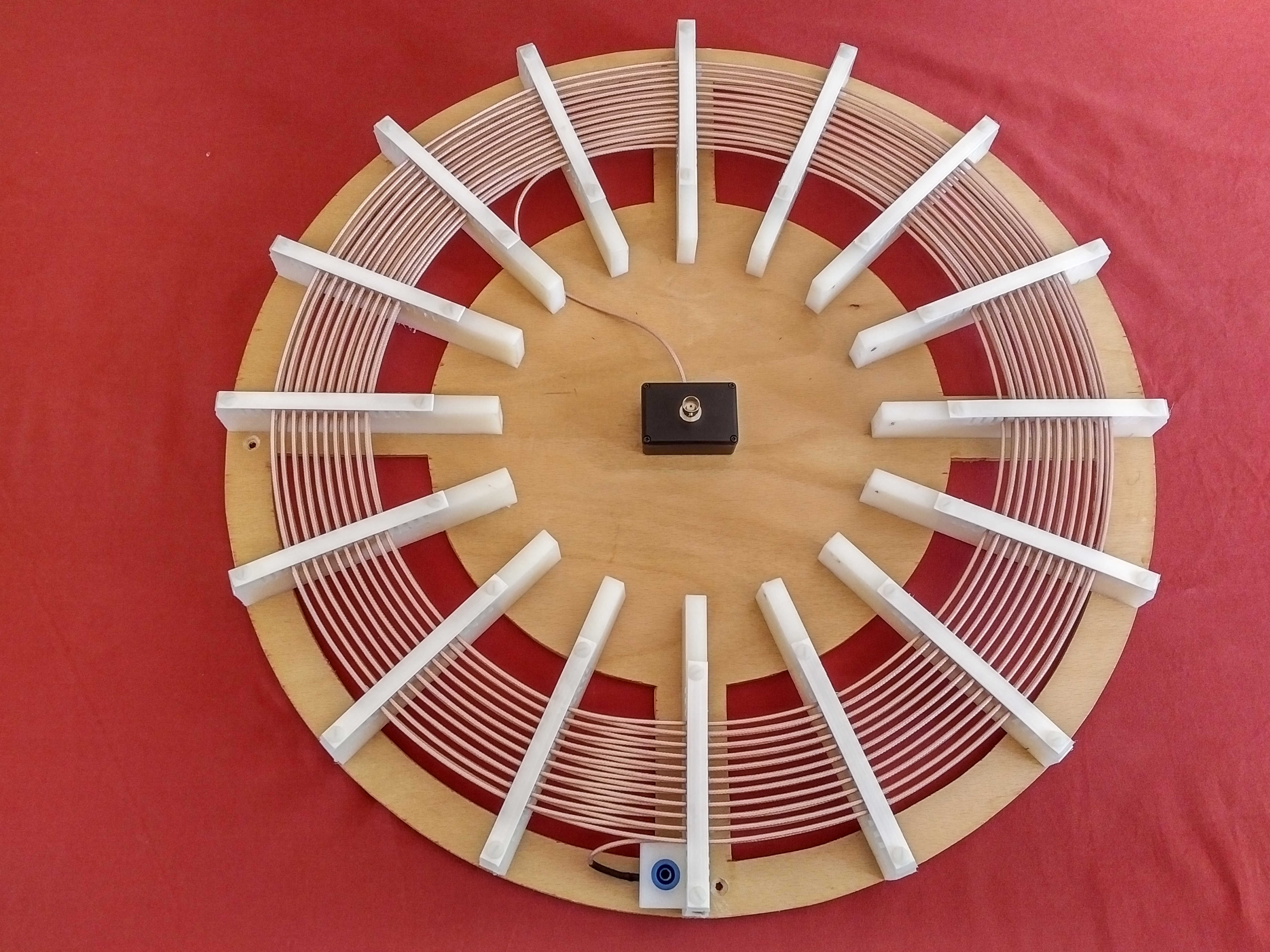
Taking into account the described considerations, and when the impedance of the coil bottom-end is lowered by an external length of wire (~2m in length) to establish the correct quarter wave coil mode of operation, the frequency at which the 180^o phase change occurs in the impedance of the coil was found to be 2400kc/s. When tuned and loaded with the methods described above this has been found to yield a fundamental resonant frequency within the stated required 160m band. With this point established the required wire length of the secondary was determined to be ~25m in length, arising from 2 layers of 10 turns inter-leaved in close coupling to form a 20 turn secondary coil, and with the following calculated dimensions. A spiral calculator tool^[8] was used to confirm these dimensions and wire length before final design and construction of the secondary coil as shown in Fig. 2.

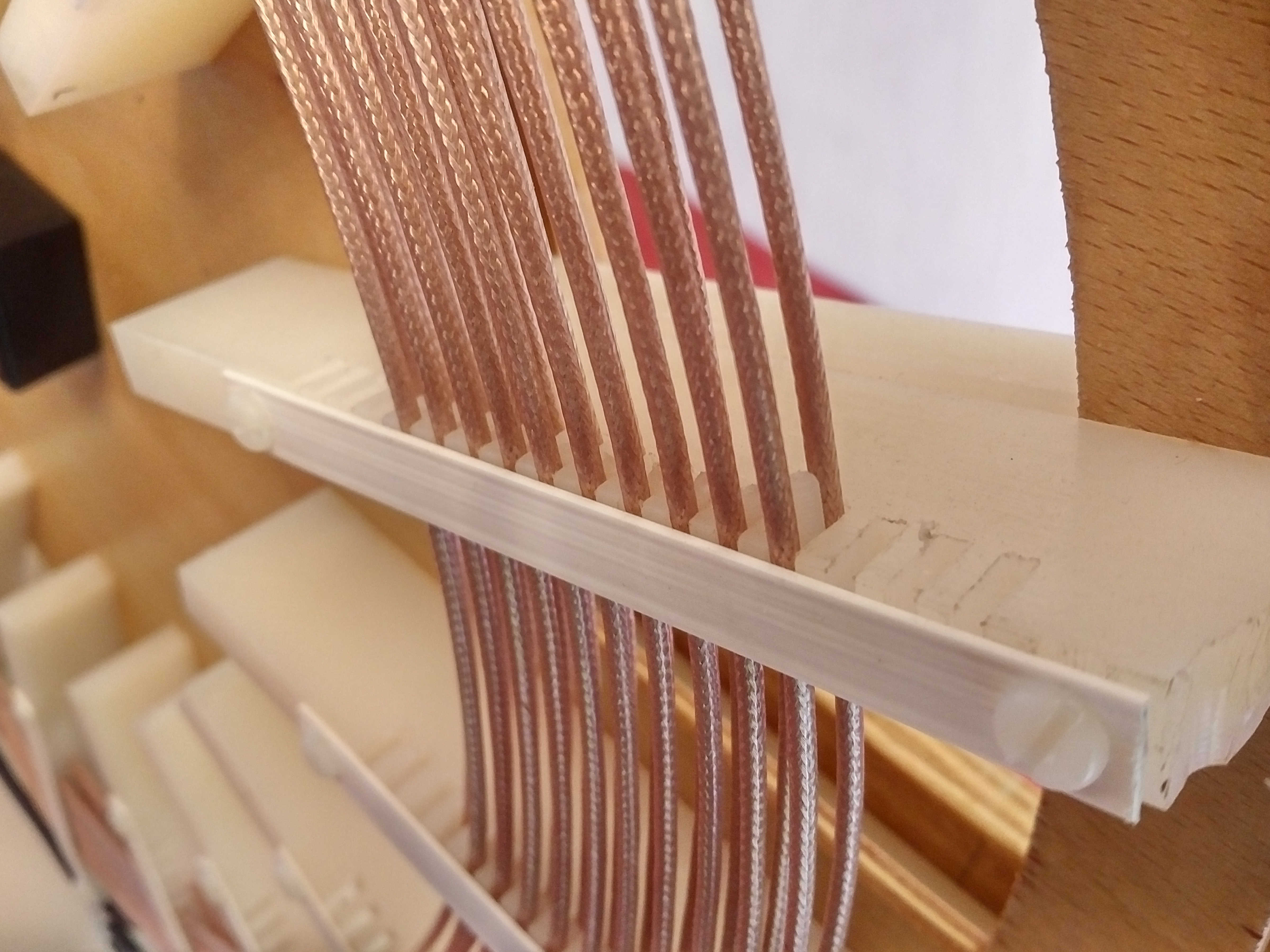
From Fig. 2. two layers of the secondary coil result in a wire length of 25.132m and a secondary conductor wire to spacing ratio of 1:3.2, a ratio that has been empirically found to benefit the formation of the Longitudinal Magneto Dielectric (LMD) wave in this geometry of coil.

The number of turns in the secondary is kept low, in this case 20 turns, in order to minimise excess voltage magnification and step-up which can cause the breakout of discharge streamers from the top load. For the purposes of the investigation of electric displacement of power it is preferred to maximise the generation of the Longitudinal Magneto Dielectric (LMD) wave, and for the case of transference the Transverse Electromagnetic (TEM) wave, by containing as much energy within the secondary as possible, and so avoiding the dissipation of energy by discharge to the surrounding environment.

This concludes the first part of the design of a suitable flat coil, and to be continued in part 2 where the properties of the secondary coil are used to consider the design requirements of a suitable primary coil.

Click here to continue to part 2 of the flat coil design.

---

1. Tesla, N., System of transmission of electrical energy, US Patent US645576A, March 20, 1900.

2. Dollard, E. & Lindemann, P. & Brown, T., Tesla’s Longitudinal Electricity, Borderland Sciences Video, 1987.

3. Mackay, M. & Dollard, E., Tesla’s Radiant Matter Replication, 2013, Gestalt Reality

4. Tesla, N., Colorado Springs Notes 1899-1900, Nikola Tesla Museum Beograd, 1978.

5. Resonance in Series-Parallel Circuits, Chapter 6 – Resonance, All About Circuits

6. Corum, K. & Corum, J., RF Coils, Helical Resonators and Voltage Magnification by Coherent Spatial Modes, TELSIKS University of Nis, Sept. 19-21, 2001.

7. Knight, D., The self-resonance and self-capacitance of solenoid coils, July 12, 2013, G3YNH

8. Bell, S., Flat Spiral Coil Calculator, DeepFriedNeon

9. A & P Electronic Media, AMInnovations by Adrian Marsh, 2019,  EMediaPress

10. Dollard, E. and Energetic Forum Members, Energetic Forum, 2008 onwards.

---

The final coil required for the purpose of experiments to be undertaken in the displacement and transference of electric power, is a loosely coupled air core resonant transformer, or what has become known as a “Tesla Magnifying Transmitter” (TMT), sometimes also referred to as a “Magnifying Transformer” (MT), and described in more detail by Tesla^[1,2], and notably through subsequent investigations by Dollard^[3], amongst others.

In the TMT the properties of both the secondary and primary have been carefully arranged empirically to be beneficial to the overall transmission of electrical energy, both in conveying power between the primary and the secondary, and most importantly in the formation of an electrical cavity between the extra coil top-load, (secondary in the case of our flat coil), and any connected transmission and/or load elements. It is to be considered that the formation of an electrical cavity constitutes one of the key important pre-conditions for the generation of a displacement event.

With the basic secondary geometric specification defined in part 1, the design of the primary can now be considered. The overall electrical characteristics and performance of the final coil are defined by first, the individual properties of both the primary and the secondary, and secondly, on their combined electrical coupling together.

Accordingly the design of the primary coil needs to take into account a wide range of factors, including:

1. The continuity and coherence of the electric and magnetic fields of induction between the primary and the secondary.

2. The inductance and series resistance of the primary coil, and hence the magnitude of current in the primary from the generator.

3. The self-capacitance of the primary, and hence its fundamental self-resonant frequency.

4. Additional parallel loading capacitance, and hence tuning of the final flat coil.

5. The number of primary turns, and in specific relation to the number of secondary turns coupled together to form a transformer.

6. The coupling factor and the fundamental resonant frequency of both the primary and secondary together.

7. The magnitude of the electric power to be passed from the primary to the secondary.

8. The geometry and materials used in construction of the primary.

9. The wire type used for the primary e.g. magnet wire, insulated multi-stranded, copper tubing, copper strip etc.

The continuity and coherence of the electric and magnetic fields of induction between the primary and secondary coils is a critical factor in generating suitable currents, (oscillating and impulse), which are required for the effective generation of significant and measurable displacement events. It is suggested that a displacement event requires the electric field of induction to be spatially in phase with the magnetic field of induction, which is not a condition that normally occurs with these two fields in processes involving transmission of electric power through transference. In relation to the purpose of the work being undertaken in this research suitable further understanding to the detail pertaining to this field can be found in the work of Steinmetz^[4,5], and Dollard^[6-9].

Transference gives rise to the normal process of electromagnetic propagation and induction, a process involving the transformation though induction of one field to another though time. This process leads to the transmission of electric power between two or multiple points where the electric and magnetic fields of induction are spatially separated at right-angles and whose magnitude will decay over time in normal processes that lead to dissipation of the two fields through the medium, system, or circuit of interest. The perceived properties of transference result in the qualities widely observed in electromagnetic propagation (e.g. through Hertzian waves), in transmission lines, and through induction and conduction of electric power (electricity) in suitable electric and electronic circuits. This field is of course vast, greatly investigated and documented, with established theory at both the macroscopic and microscopic levels which can easily be corroborated and confirmed both by practical experiments, and the vast implementation of electric and electronic devices within industry.

In stark relation to this the displacement of electric power stands in its infancy, is generally not well investigated, understood, or even carefully and systematically investigated. This would appear to result both from the practical difficulties in generating and then measuring the properties of this state, and also from the lack of development and interest from industry, and since early postulation and investigation by the such notable figures such as Maxwell^[10], Heaviside^[11], Steinmetz^[4,5], and Tesla^[12].

It is suggested that the displacement of electric power results from a coherent relationship between the electric and magnetic fields of induction, in such a way that they cannot easily be distinguished as separate fields by conventional measurement means. If this were the case then both these fields would appear undifferentiated from one another, or rather in a cooperative relationship where both are in phase spatially and temporally. In this way the displacement of this “combined” field could occur over any distance without either constituent field dissipating, as there is no required transformation from one field to another in order to “propagate” or “transmit” from one position to another. The properties arising from this coherent and cooperative relationship between the two fields should be observable, under the correct and necessary pre-conditions, as displacement events which give rise to unusual and yet to be explored electrical phenomena that are not explainable by normal modes of transference.

It is conjectured that the displacement of electric power results from the impact of a non-linear event on the coherent relationship between the two fields of induction. At its very root where there is no distinct differentiation between these two fields, they are undifferentiated, a state that we cannot observe electrically by normal perceptual or measurement means. As the process of differentiation occurs between the fields there is as yet a coherent and cooperative inter-dependent relationship between the two forming fields, and they are taking a path of becoming less non-linear and more linear to our perceptual observation. This inter-dependent state should be observable when the correct pre-conditions have been established and a non-linear change is introduced to the system. This non-linear change initiates a displacement event where the resulting change to the energetic dynamics of the system give rise to electrical phenomena that can be measured through the linear process of transference, that is, with normal voltage and currents. The process of transference results from the full and linear separation between the electric and magnetic fields of induction as a response to the displacement event.

The process of displacement is often likened to establishing a longitudinal wave, (a condition between the two fields of induction), often referred to as a standing wave within an electrical system bounded in a specifically terminated cavity e.g. two joined TMTs either by a conducting medium such as a wire or through the earth. It is suspected, and to be determined, that the longitudinal wave, or standing wave case, is actually a pre-condition to a displacement event rather than the event itself. Establishing a standing-wave in a TMT cavity results in a different set of properties from displacement, where the electric and magnetic fields of induction are not spatially or temporally in phase and hence no power is dissipated, but where the two fields of induction are balanced but still in the fully linear state of transference. This means that a longitudinal wave, or an LMD standing wave, must first be established as a pre-condition within the system, and then a non-linear change introduced to this system as a trigger for the generation of a displacement wave. The generation of a displacement wave changes the energetic dynamics in the system to re-establish the balance of the magnetic and electric fields of induction, and hence re-establish the “harmonious” steady-state of the system having addressed the change or “need” of this system.

With all this said regarding displacement and transference it is critically important in the design of our MT, for the purpose of investigating displacement events, to ensure that we create a system which is best suited to sustain for as long as possible the coherent balance and continuity between the electric and magnetic fields of induction. In this way we so arrange our design to ensure that any generated displacement events occurring from or within the generator, from or within the medium conveying the electric power, and from or within any load thus designed to receive or utilise this power, will sustain the event for as long as possible and with amplitude such that it can be investigated and measured. Tesla^[12] suggested and established this requirement clearly, in that the conducting boundary conditions for the electric and magnetic fields of induction must ensure the maximum balance, continuity, and coherence for these two inter-dependent fields when moving from one section of an electrical system to another. In this way he established the requirement between the primary and secondary of an MT should be made from equal weights of conductor.

From further investigation by others, notably Dollard^[3,6], where the density of the conductor in the primary and secondary is the same, (e.g. for a primary and secondary both with copper as the conductor), equal volumes of the conductors can be considered equivalent to equal weights of the conductors, and has been found to apply best when working at lower frequencies where the skin effect does not have a significant effect on the impedance of the conductor, e.g. when working with normal copper or aluminium conductors at a frequency < 3000kc/s. At higher frequencies where the skin-effect can dominate the impedance of the conductor, balancing the bounding conditions for the two fields of induction can be better accomplished by equal surface area of the conductors.

Fig 2. below shows the effects of the skin-effect on the penetration depth with frequency for a range of common conductors.

In the case of the current flat coil design operating at nominally the loaded fundamental resonant frequency in the range 1810 – 2000kc/s, with both copper in the primary and secondary, equal weights calculations have been used to design the primary using multi-stranded wires, braided coaxial shields, copper tubing, and copper strip.

The design of the current flat coil primary is concluded in part 3 with consideration to these different types of primary conductor, and the calculations as to size and length of the conductor to be used for equal weights of conductor in the secondary and primary coils.

Click here to continue to part 3 of the flat coil design.

---

1. Tesla, N., Apparatus for Transmitting Electrical Energy, US Patent US1119732A, January 18, 1902.

2. Tesla, N., Rare Notes from Tesla on Wardenclyffe, Electric Spacecraft, 26, Apr/May/Jun 1997.

3. Dollard, E., Condensed Intro to Tesla Transformers, Borderland Sciences Publication, 1986.

4. Steinmetz, C., Theory and Calculation of Transient Electric Phenomena and Oscillations, McGraw-Hill Publication, 1909.

5. Steinmetz, C., Elementary Lectures on Electric Discharges, Waves and Impulses, and Other Transients, McGraw-Hill Publication, 1911.

6. Dollard, E., The Oscillating Current Transformer, JBR, May-June 1986.

7. Dollard, E., Theory of Wireless Power, Borderland Sciences Publication, 1986.

8. Dollard, E., Symbolic Representation of Alternating Electric Waves, Borderland Sciences Publication, 1986.

9. Dollard, E., Symbolic Representation of the Generalized Electric Wave, Borderland Sciences Publication, 1986.

10. Maxwell, J., A Dynamical Theory of the Electromagnetic Field, Phil. Trans. Royal Society, pg459-pg512, January 1865.

11. Heaviside, O., Electrical Papers, Vol I & II Macmillan and Co., 1892.

12. Tesla, N., Colorado Springs Notes 1899-1900, Nikola Tesla Museum Beograd, 1978.

13. A & P Electronic Media, AMInnovations by Adrian Marsh, 2019,  EMediaPress

14. Dollard, E. and Energetic Forum Members, Energetic Forum, 2008 onwards.

---

Following on from part 2 of the flat coil design it has been establised that the primary and secondary coils will be so arranged to contain equal weights of conductor, dependent on the geometry of the specific conductors being used, and so to ensure the continuity of conductor boundary conditions and hence the balance, continuity and coherence of the electric and magnetic fields of induction between the primary and the secondary coils.

It is important in the primary to maximise the current carrying capability of the coil, which will allow the generator or tank circuit to provide strong oscillations, bursts, and impulses, according to the type of experiment to be undertaken. This means that the inductive reactance of the primary should be as low as possible within the band of frequencies required, allowing a large current to flow, and whilst also allowing for a practical value of tank capacitor with sufficient adjustment to tune above and below the frequencies of interest. In this case it is intended to use a variable high voltage vacuum capacitor in the range 100pF – 1500pF, with the desired fundamental resonant frequency change at 2400kc/s occurring at a tank capacitance in the range 900pF – 1100pF which allows for good adjustment for the variable vacuum capacitor, but also for the ease of use of a fixed high voltage capacitance of 1000pF (1nF). For the tank capacitance to be 1000pF, and in the ideal theoretical case, the  inductance of the primary would be 4.4uH.

Accordingly, and in consideration of the 20 turns in the secondary designed in part 1, the number of turns in the primary will be fixed at nominally 2, and with the ability to tap the primary, (for use with bare metal primary materials only e.g. copper tube or strip), slightly above or below the exact 2 turns mark should a finer resolution of tuning be required. This gives a voltage magnification in the magnifying transformer according to the secondary-primary turns ratio of 10, which is high enough to magnify the generator voltages to a more usable level in the observation and measurement of displacement events, and yet still low enough to allow high voltage generators to be used in the tank circuit without causing excessive breakout and discharge, and hence dissipation of energy to the surrounding environment, from the secondary.

Wire spacing between the turns of the primary is to be arranged to avoid any possibility of electric discharge through sparking when the primary is driven at resonance from a high voltage generator such as a vacuum tube oscillator or linear amplifier, a static or rotary spark gap generator, or other high voltage generator such as a vintage diathermy machine or electro-therapy generator. This means that the wire spacing in the primary should be safe for potentials up to 20kV applied across the primary terminals by a generator, and contacts to the primary and the primary conductor size should be able to support total input powers up to 2.5kW. With this considered the nominal distance between the start of the outer turn and the end of the second inner turn was set at 25mm, which gives a turn spacing of 12.5mm. The generally accepted dielectric strength of air at normal temperature, pressure, and humidity is 30kV/cm. When using a bare copper 3/16″ or 4.8mm tube this leaves the gap between conductors in the primary of 7.7mm which would have a nominal breakdown voltage in air of ~ 23kV, which is considered adequate for the highest voltage generators currently used in this research. The centre diameter of the primary coil was determined empirically by adjustment in relation to the secondary where the Q of the final coil was maximised, and a coupling factor between the primary and most outer turns of the secondary of ~ 0.15 was achieved.

With these characteristics defined the primary wire length could be defined to best match the required characteristics. Again the spiral coil calculator was used to assist in this calculation:

From Fig. 1. the required primary coil wire length is 3.455m, which theoretically yields a coil inductance of 4.8uH. At 2400kc/s for the desired fundamental resonant frequency phase change this yields a tank capacitance of 914pF, which is within the range required in the flat coil design.

Conductors to be used / tested in the secondary coil include:

1S. PTFE / Teflon coated, silver plated, multi-stranded wire. The strong PTFE coating prevents spark or streamer breakouts from running along the length of the wire, and the silver coating bonds the jacket firmly to the inner wire conductor. Given the secondary coil properties, dimensions, and turn spacing required the wire selected as the most suitable was: Awg16, 19/0.3 (19/29), ID ~ 1.35mm, OD ~ 2.5mm, white PTFE jacket.

2S. Silicone coated, flexible high density micro-stranded wire. The high number of conductor strands make this wire suitable for a higher frequency, lower-loss winding, and the silicone coating makes the wire very flexible with good high voltage and temperature properties. Given the secondary coil properties, dimensions, and turn spacing required the wire selected as the most suitable was: Awg16, 252 strands, ID ~ 1.5mm, OD ~ 3.0mm, black silicone jacket.

3S. Braided shield coaxial cable. The outer shield to be used as the conductor with many strands maximising the inter-turn capacitance, and the conductor surface area, and with the inner coaxial conductor non-connected. Given the secondary coil properties, dimensions, and turn spacing required the wire selected as the most suitable was: RG316 Coaxial cable OD ~ 2.50mm, transparent Teflon jacket.

Conductors to be used / tested in the primary coil include:

1P. Silicone coated, flexible high density micro-stranded wire. The high number of conductor strands make this wire suitable for a higher frequency, lower-loss winding, and the silicone coating makes the wire very flexible with good high voltage and temperature properties.

2P. Flexible copper tubing, with good high current capability and easy primary tapping to the bare conductor surface.

3P. Copper strip, with high surface area, high current capability, and highest Q for the high frequency experiments.

The early versions of the flat coil used wire combination 1S-1P for both the generator and load coil, providing an easy to use coil structure suitable for a wide range of preliminary investigations into the displacement and transference of electric power. This was later replaced by 1S-3P as the best measured for both the generator and load coil for experiments with displacement events. Later experiments in telluric transmission of electric power used the 1S-3P combination as the best measured generator coil, and with 3S-1P as the best measured load coil. The details of these measurements and there results will be reported in the experimental posts.

For calculations of copper weight, volume, and other useful data with respect to solid and stranded wires, and where either exact specification data, or measured data, is not available for the actual wire used, the following wire and cable data from Calmot can be used.

Click here to view or download the Calmot wire and cable data.

1. For coil 1S-1P the equal weight of copper calculation:

Secondary wire length (from part 2): 25.132 m

Specification unit weight of actual wire used: 11.120 kg/km

Secondary wire weight = 11.120 x 25.132 / 1000 = 0.279 kg

Calmot data for 8 AWG 1666 / 40: 81.1 kg/km

Actual primary wire 1P 8 AWG 1600 / 40 = 1600 / 1666 x 81.1 = 77.887 kg/km

Required primary wire length for exact equal secondary and primary weights = 0.279 x 1000 / 77.887 = 3.582 m

Calculated primary wire length from flat spiral coil calculator in Fig. 1: 3.455 m

1P Primary wire length of silicone coated micro-stranded 8 AWG 1600 / 40 = 3.58 m

2. For coil 1S-2P the equal volume of copper calculation:

Secondary wire weight (as above) = 0.279 kg

Measured unit weight of pure copper pipe OD 4.75mm (3/16″), wall thickness 0.8mm: 77.420 kg/km

Required primary wire length for exact equal secondary and primary weights = 0.279 x 1000 / 77.420 = 3.603 m

2P Primary length of 4.75mm (3/16″) pure copper pipe = 3.60  m

3. For coil 1S-3P the equal weight of copper calculation:

Secondary wire weight (as above) = 0.279 kg

Specification unit weight of pure copper strip 30mm wide and 0.3mm thick (standard strip available): 80.450 kg/km

Required primary strip length for exact equal secondary and primary weights = 0.279 x 1000 / 80.450 = 3.467 m

3P Primary length of 30mm x 0.3mm pure copper strip = 3.47  m

4. For coil 3S-1P the equal volume of copper calculation:

Measured unit weight of RG316 outer braid only: 6.150 kg/km

Secondary wire weight = 6.150 x 25.132 / 1000 = 0.155 kg

Actual primary wire 1P 10 AWG 1050 / 40 = 45.150 kg/km

Required primary wire length for exact equal secondary and primary weights = 0.155 x 1000 / 45.150 = 3.433 m

1P Primary wire length of silicone coated micro-stranded 10 AWG 1050 / 40 = 3.50 m (2% error to allow for 2 complete turns and connection)

All required primary lengths, (other than case 4 where the primary must be extended for 2 complete turns), are longer than the flat spiral coil calculation of 3.455m, which allows for 2 full turns of the primary and connections to be made to the primary capacitor. Connections to the primary capacitor are arranged at the point where the primary length is equal to that required to equal the weights of the secondary and primary coils.

It must also be noted that the primary capacitor introduces a weight of conductor into the primary circuit calculation which has not been accounted for above. In the experimental stage different capacitor sizes and weights will be used to determine the overall induction field mismatch caused by this circuit element and/or other elements in the generator or load. In the case of diminished displacement and transference of electric power results, the primary weight of copper will need to be adjusted through reduced AWG size (P1), reduced tube diameter (P2), and reduced strip width (P3), in order to get the best equal conductor weight match.

This concludes the three design parts for the flat coil with all the necessary parameters for construction of the final coil.

Click here to continue to the flat coil construction post.

---

1. A & P Electronic Media, AMInnovations by Adrian Marsh, 2019,  EMediaPress

2. Dollard, E. and Energetic Forum Members, Energetic Forum, 2008 onwards.

---