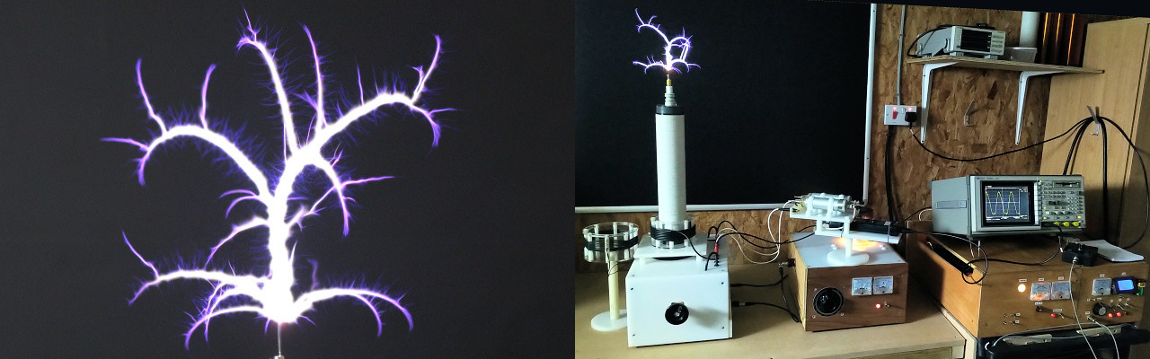
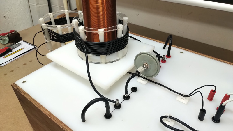
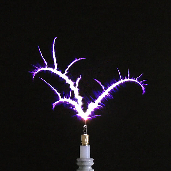
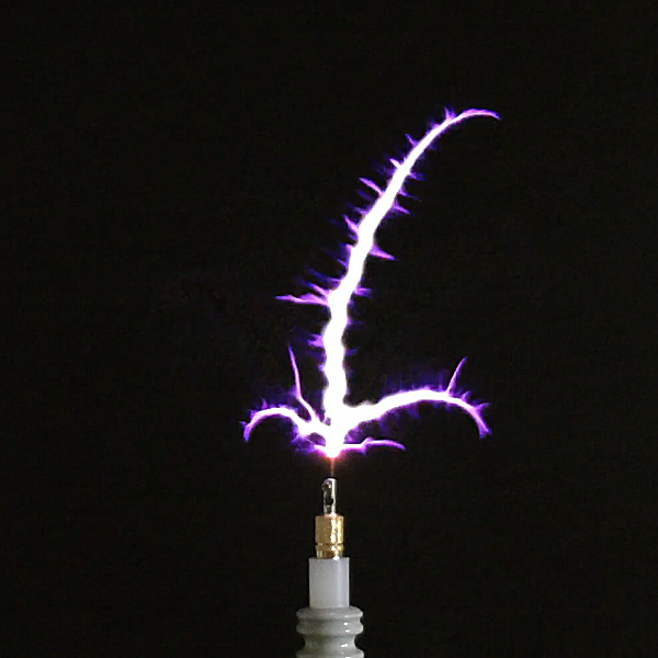
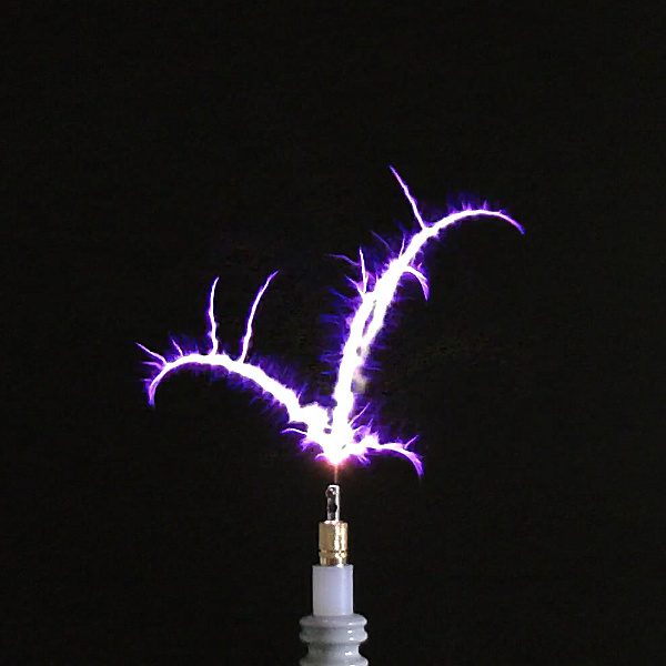
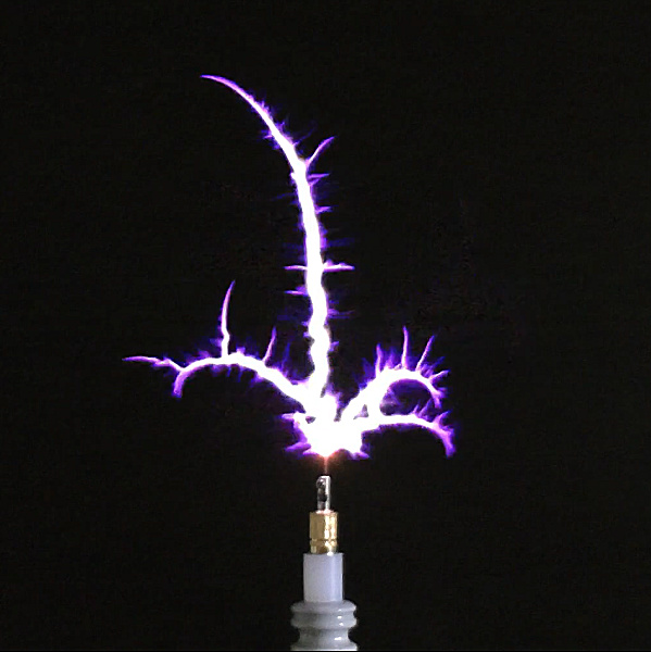
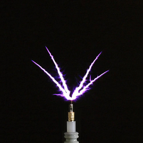
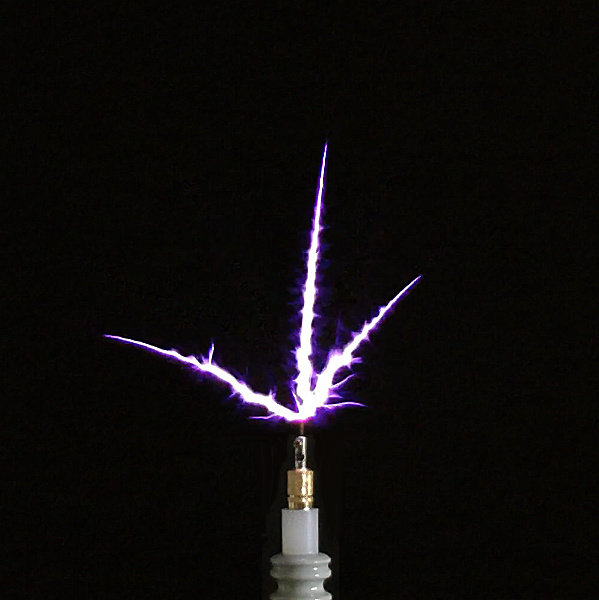
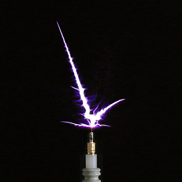
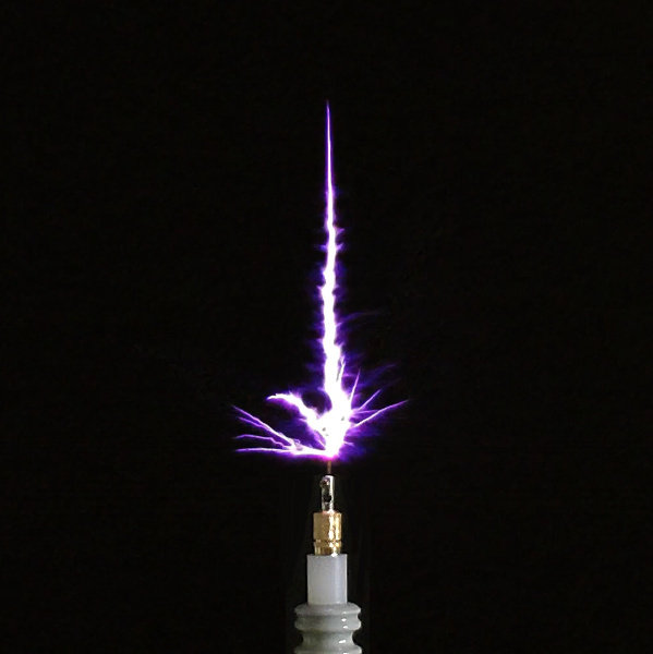
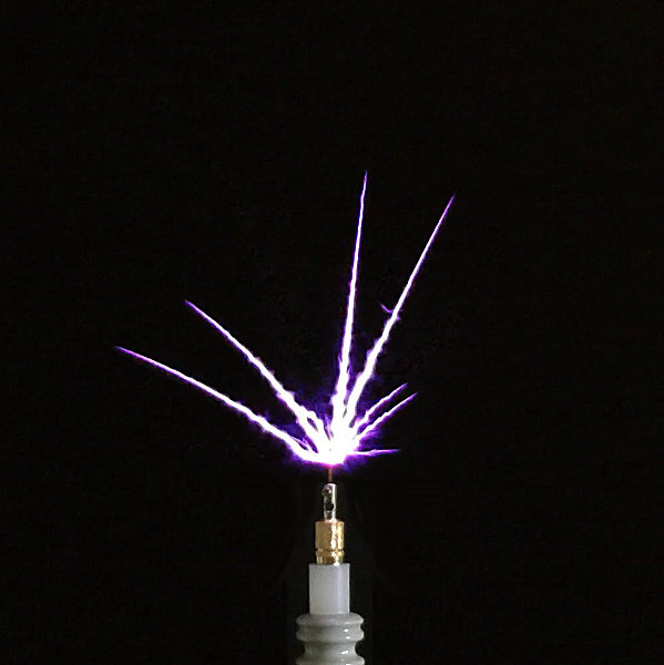
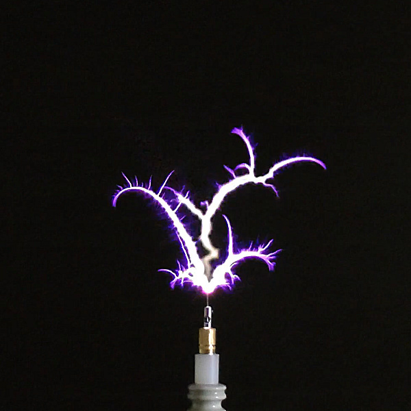
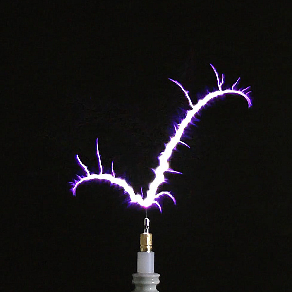
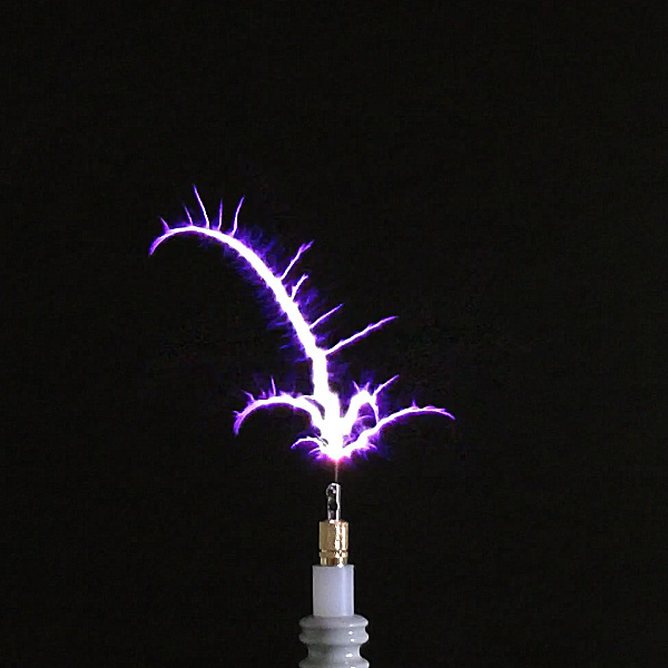
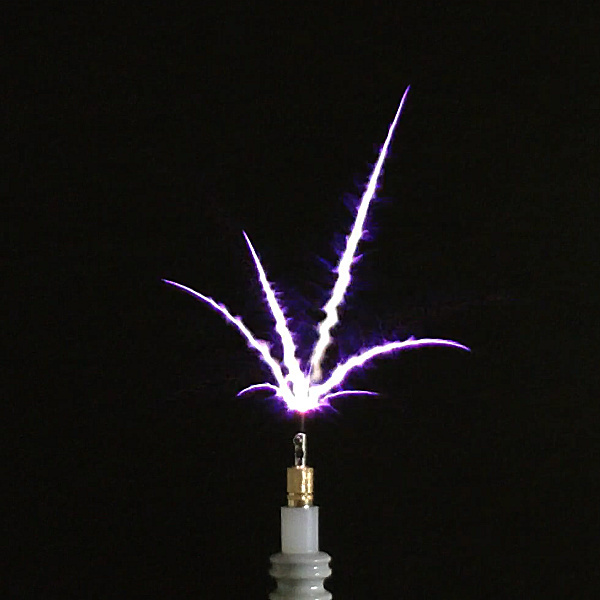
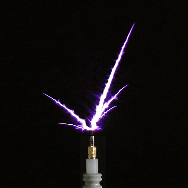
The Golden Ratio Discharge a fundamental part of The Wheelwork of Nature, revealing the underlying natural order expressed within electricity. (Click to enlarge images, and hover to pause slides)
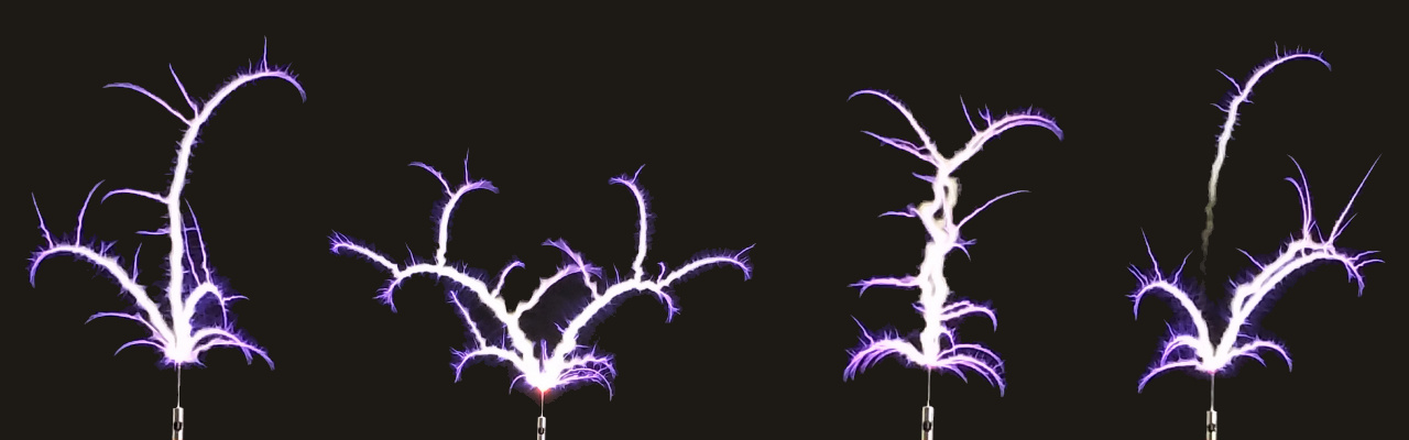
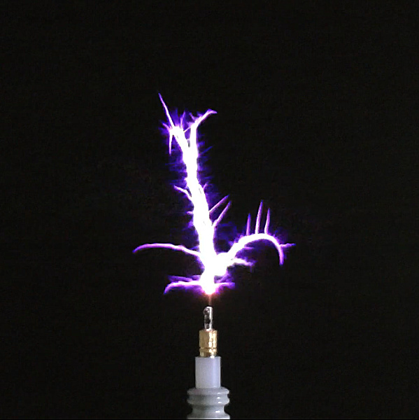
The Golden Ratio Discharge showing well defined order, symmetry, as well as spatial and temporal coherence and choreography.
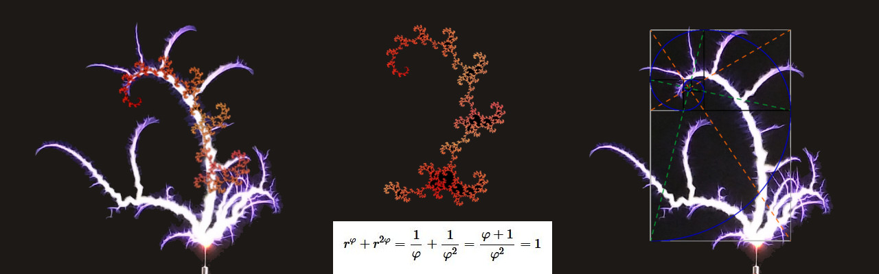
The Golden Ratio Discharge, also known as The Fractal-Fern Discharge, has its best fit in the form of The Golden Dragon, which is a fractal that expands according to the Golden Ratio.
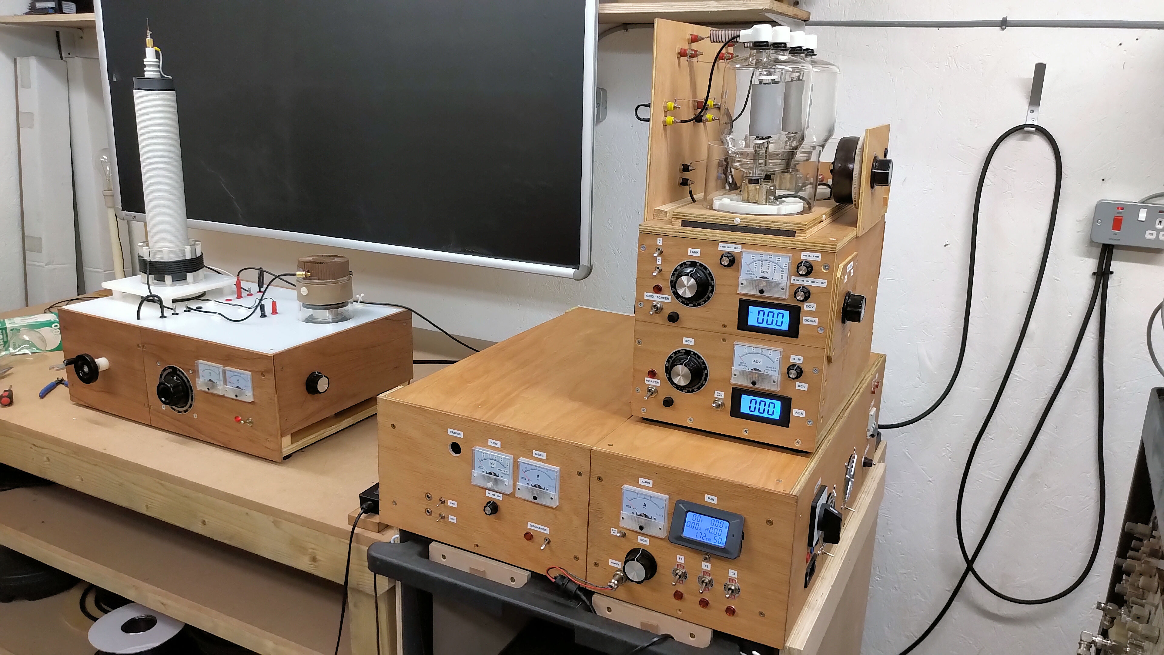
The AMInnovations MiniGen is a complete portable vacuum tube Tesla coil generator, and suitable for a wide range of different electricity experiments and demonstrations.
High-Efficency Transference of Electric Power experiments passing 500W of power across a 40awg (80 micron) single wire at an efficiency over 99.5%.
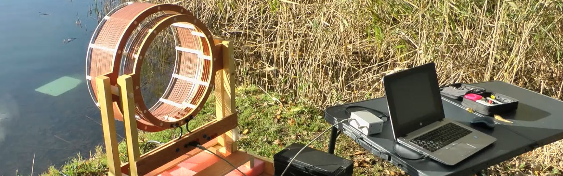
Plasma discharge, induction, and tension experiments using specialised Tesla Transformers driven by a vacuum tube generator, and similar in design to Eric Dollard's cosmic induction generator.
Experiments in the Displacement and Transference of Electric Power, using a flat-coil Tesla Magnifying Transmitter based on the design of Eric Dollard, Peter Lindemann, and Tom Brown.
A potential Radiant Energy event - a conjectured emission from Coherent Displacement in the single wire cavity of a Tesla Magnifying Transmitter with non-linear generator drive.
Displacement of Electric Power experiments using a high-energy discharge apparatus to explore non-linear displacement and disruptive phenomena, including "exploding wires", dielectric shock waves, and Tesla Radiant Energy emissions.
Telluric Transference of Electric Power experiments using a specialised Tesla Magnifying Transmitter, and measuring the proportion of telluric to radio-wave reception over 100 miles from the transmitter.
Telluric transference of electric power experiments using both two-coil and three-coil systems. The three-coil system includes Tesla's extra coil and introduces a more complex longitudinal cavity arrangement.
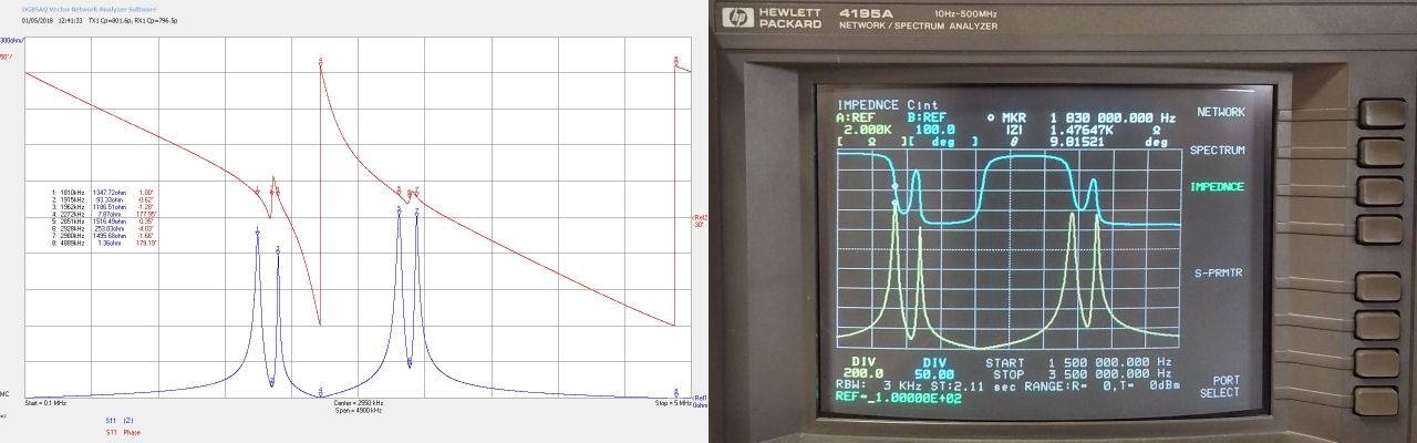
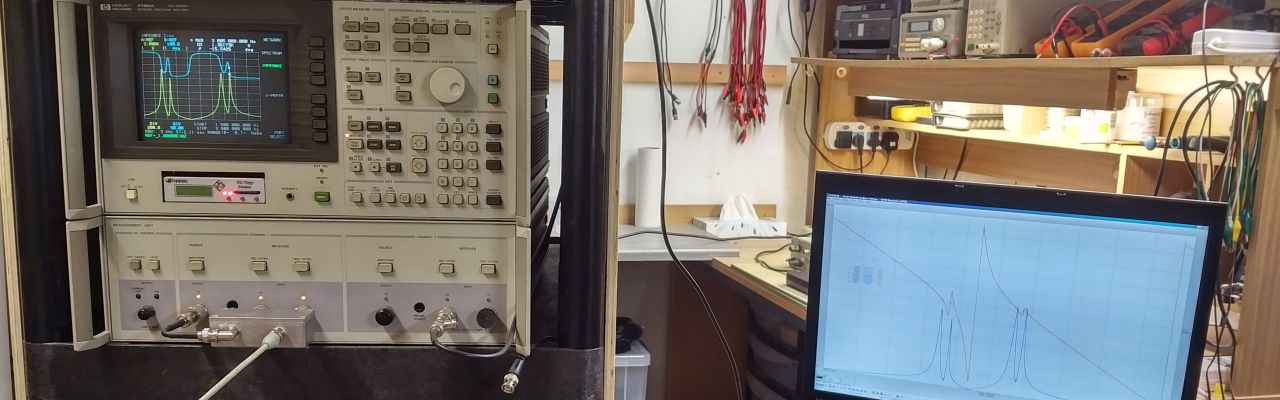
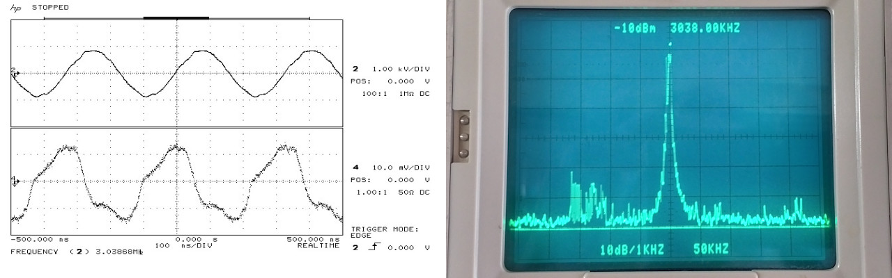
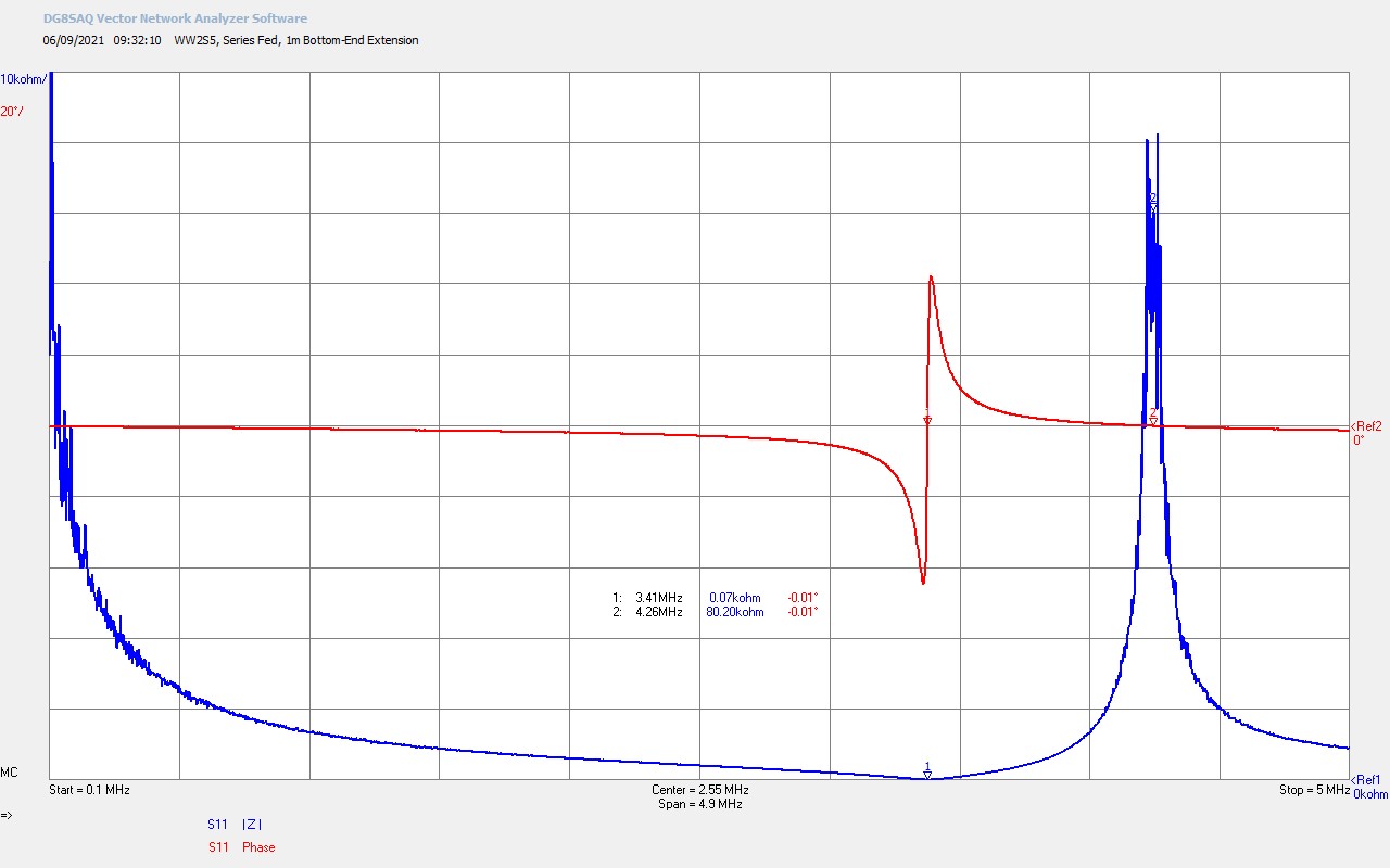
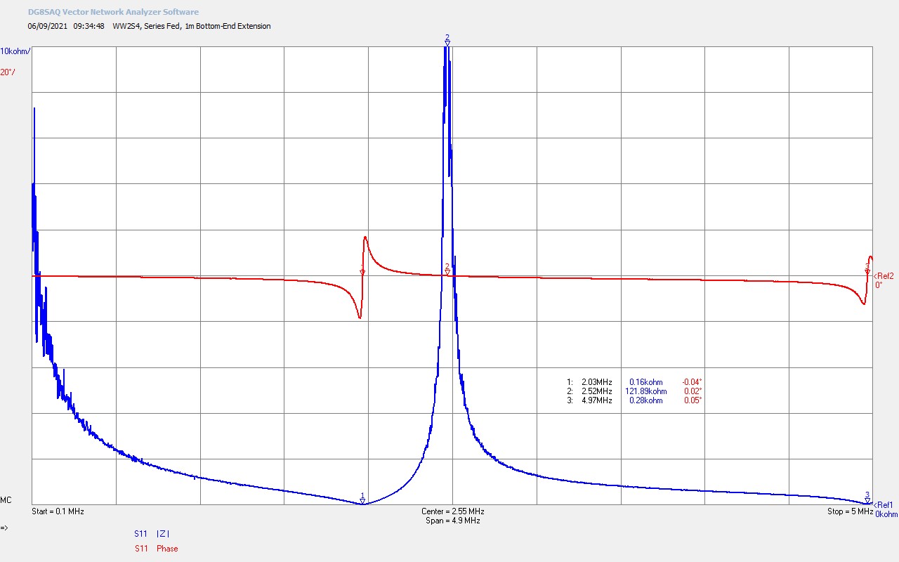
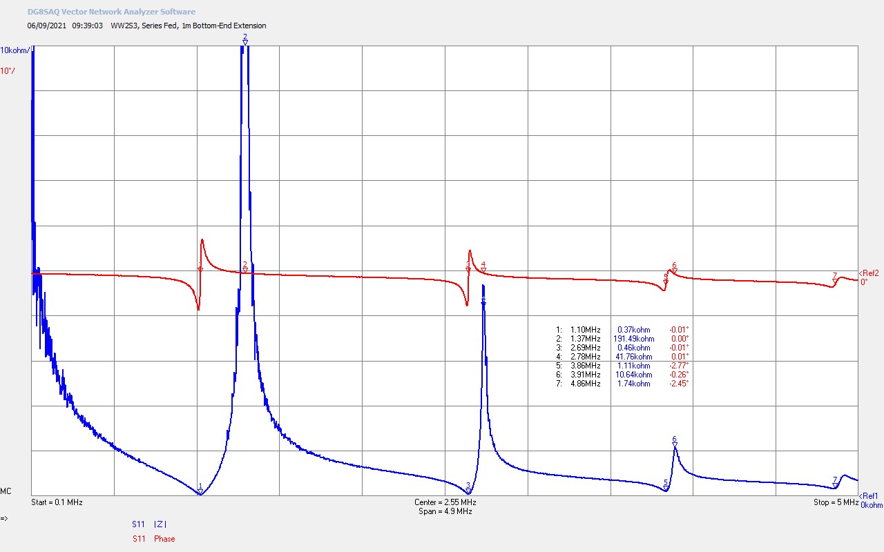
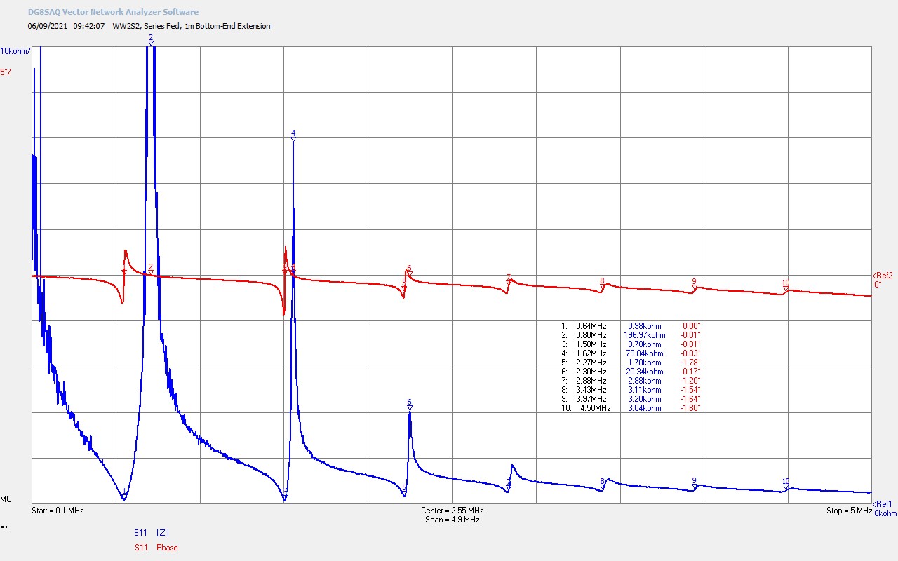
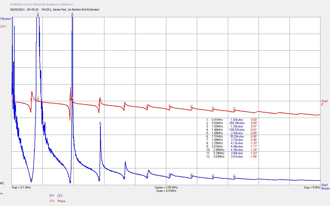
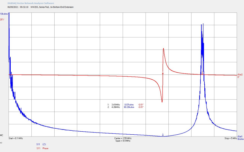
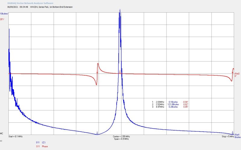
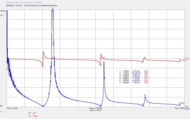
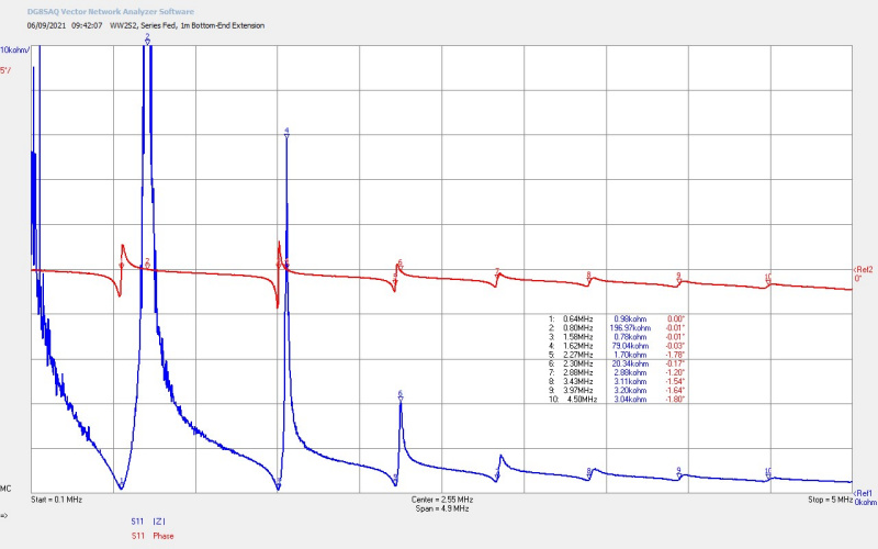
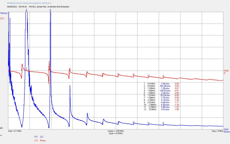
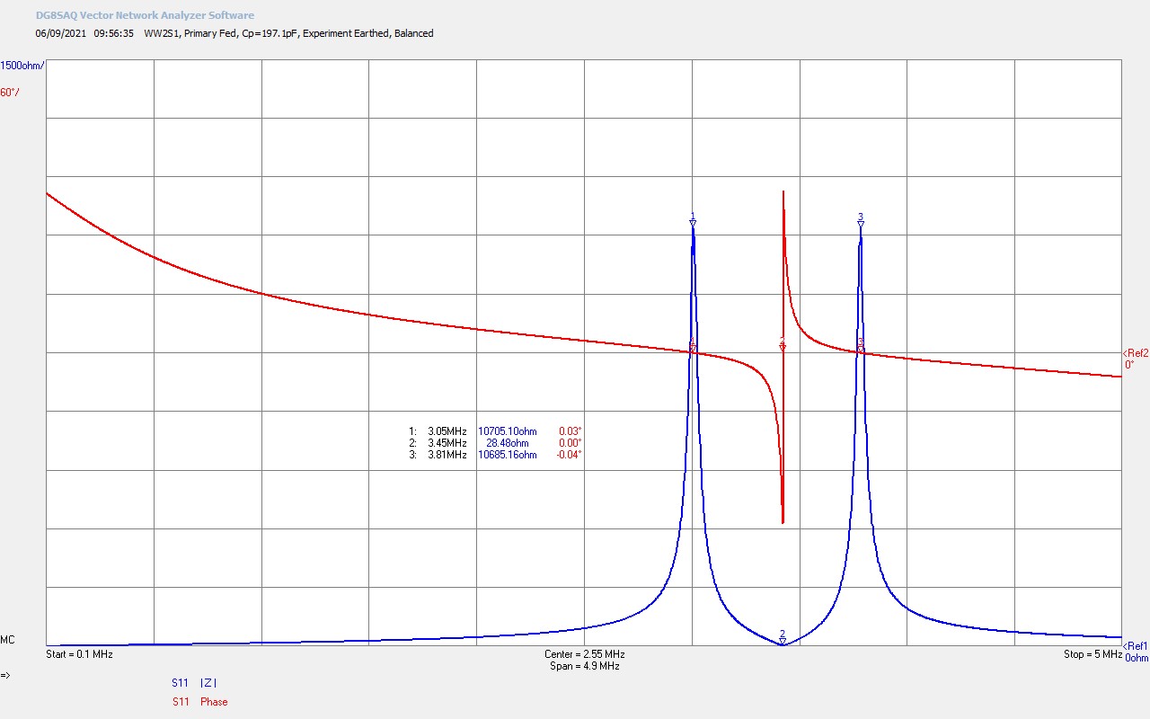
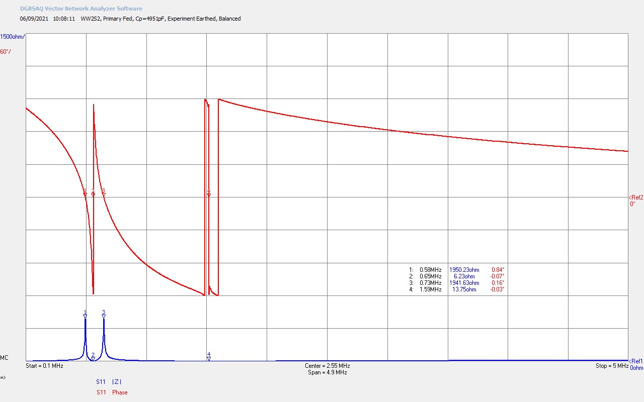
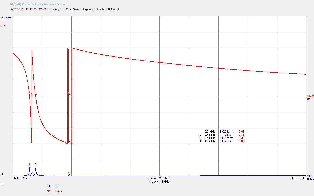
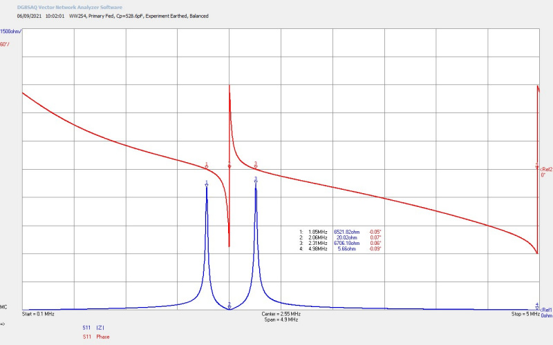
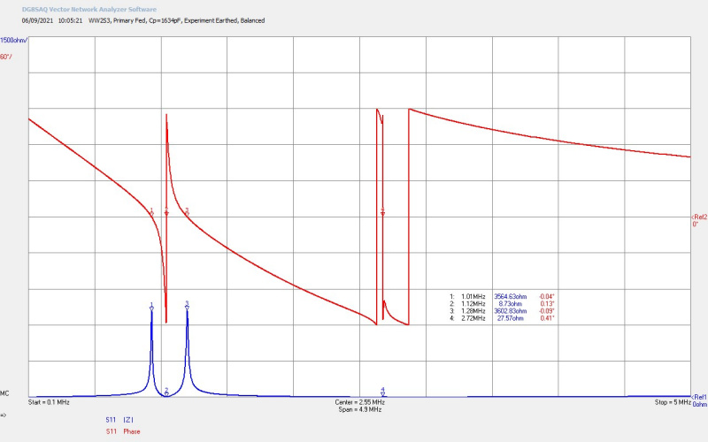
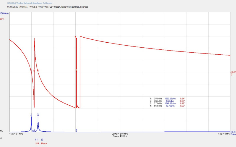
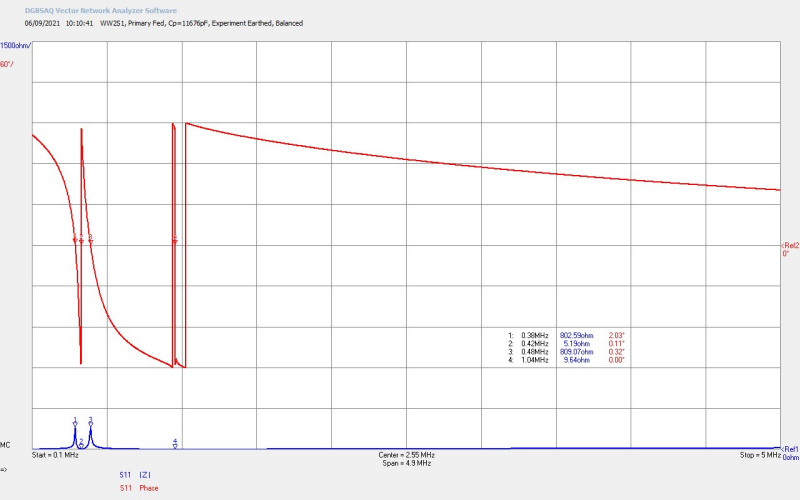
Input impedance Z11, as seen by the generator, of two flat coils bottom-end connected via a single wire cavity in a Tesla Magnifying Transmitter, and tuned to balance the Transverse and Longitudinal modes.
Input impedance frequency measurements of the twin coil experimental apparatus compared on a HP4195A and a SDR-Kits DG8SAQ VNA
Measured upper resonant frequency of oscillation for the single flat coil in Telluric electric power transmission tests.
"Electric power is everywhere present in unlimited quantities ...""Electric power is everywhere present in unlimited quantities and can drive the world's machinery without the need of coal, oil, gas ...""Electric power is everywhere present in unlimited quantities and can drive the world's machinery without the need of coal, oil, gas, or any other of the common fuels."Nikola Tesla c. 1900
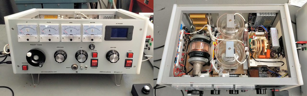
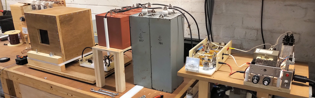
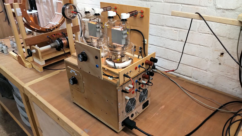
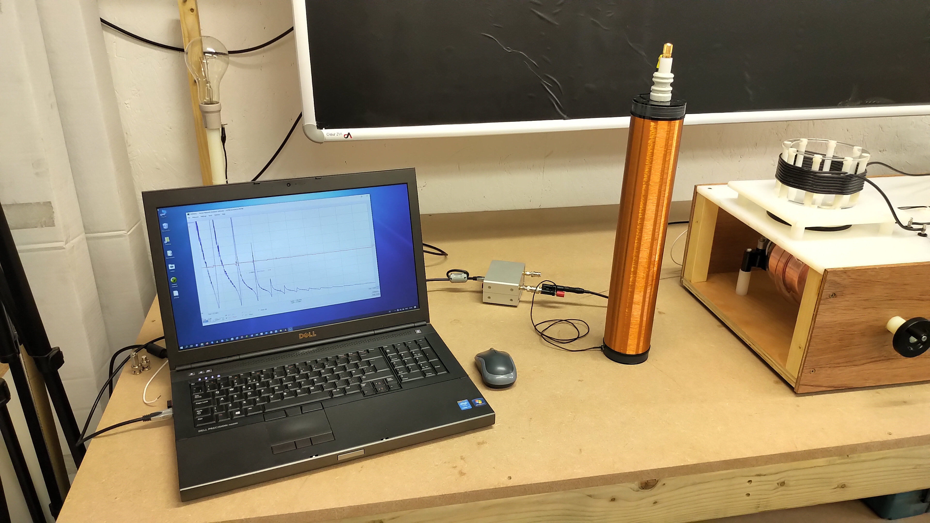
In research using Tesla coils it is inevitable that sooner or later a vacuum tube power supply will become a necessary and invaluable addition to the laboratory equipment. Vacuum tubes when correctly setup and operated are a robust and high power solution to driving Tesla coils from very low frequencies, and to well into the HF frequency band. Most of my experiments are conducted in the 160m amateur band with a centre frequency around 2Mc, and with tuning that can go down as low as 500kc, and up to almost 4Mc. A vacuum tube generator that can be flexibly configured to drive different configurations and types of tubes to power levels over 1kW, and even up to as high as 5kW, opens the door to many fascinating and unusual electrical phenomena, that can be observed and measured using Tesla coils driven at higher powers and higher frequencies. This post is the first in a sequence to look at my own tube power supply, designed specifically with rapid prototyping and Tesla coil research in mind, and is the product of using vacuum tubes of various different types and configurations in my research over the years.
Note: A high voltage supply is capable of delivering voltages and currents, even at lower powers, that are instantly lethal, and that any design and operation of a high voltage unit should be undertaken with great care by a trained and experienced individual. I have so far presented on my website a basic and yet configurable Vacuum Tube Generator based around dual 811A’s, and which has been used in a range of already reported experiments including, Transference of Electric Power, Single Wire Currents, and Tesla’s radiant energy and matter. In this post I start looking at a much more comprehensive tube power supply that I use on a daily basis with a range of different tube boards. I will be looking at the design, construction and operation of the heater, grid & screen supply (TPS-HGS), including a video overview and simple experimental demonstration of its basic operation. More detailed and sophisticated operation will be covered in subsequent experimental posts as I publish them.
Before launching into the details of this supply, I will first give an overview of my complete tube power supply system, and its major components:
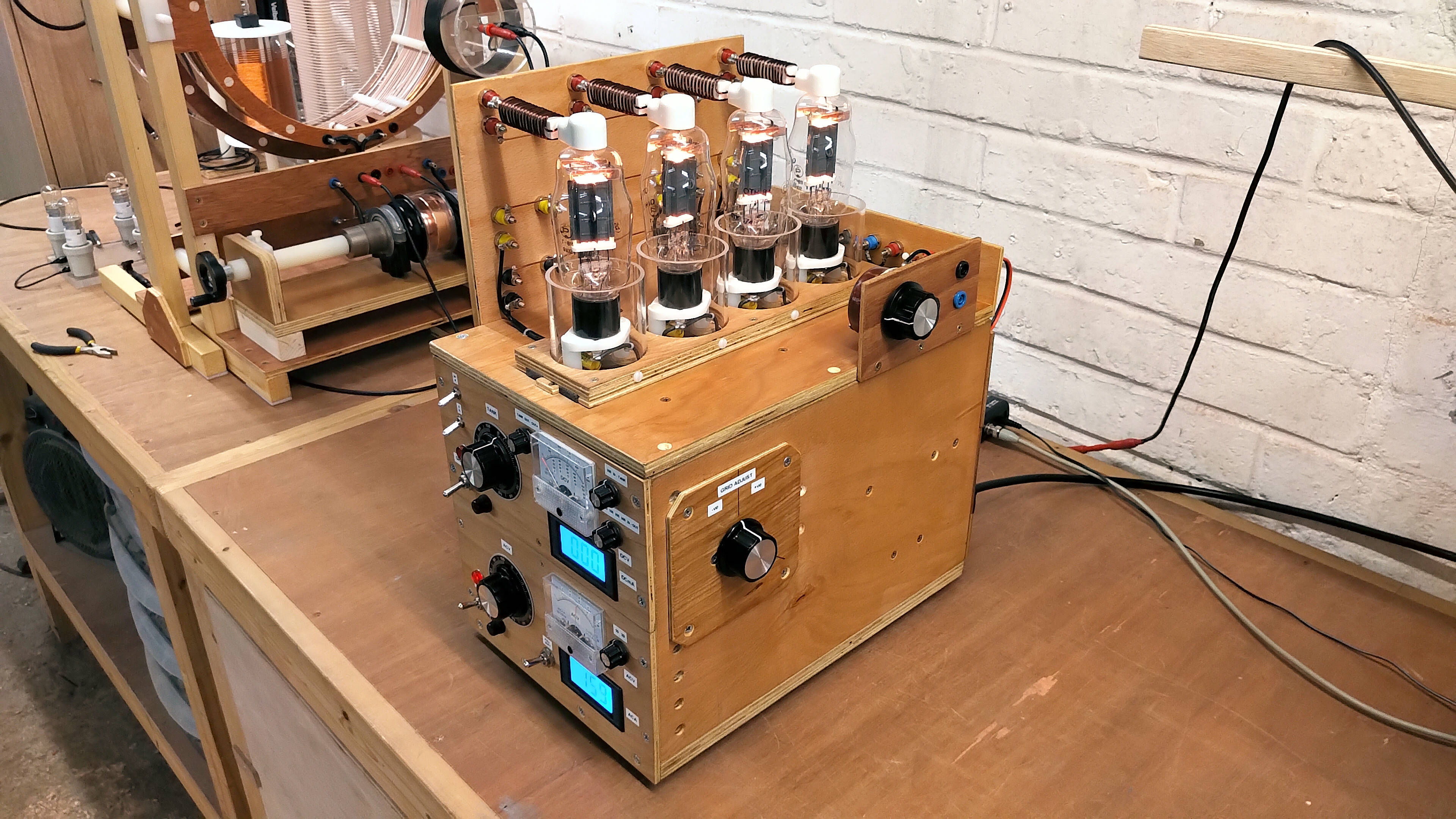
1. The heater, grid & screen supply is covered in this post, and provides the filament heater supply to the installed tube board with variable control up to a maximum 12.6V @ 25A, a finely controllable grid bias supply with wide operating characteristics between ±750V DC @ 200mA, or a finely controllable screen or auxiliary bias supply up to 1500V DC @200mA.
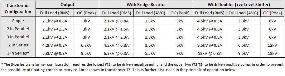
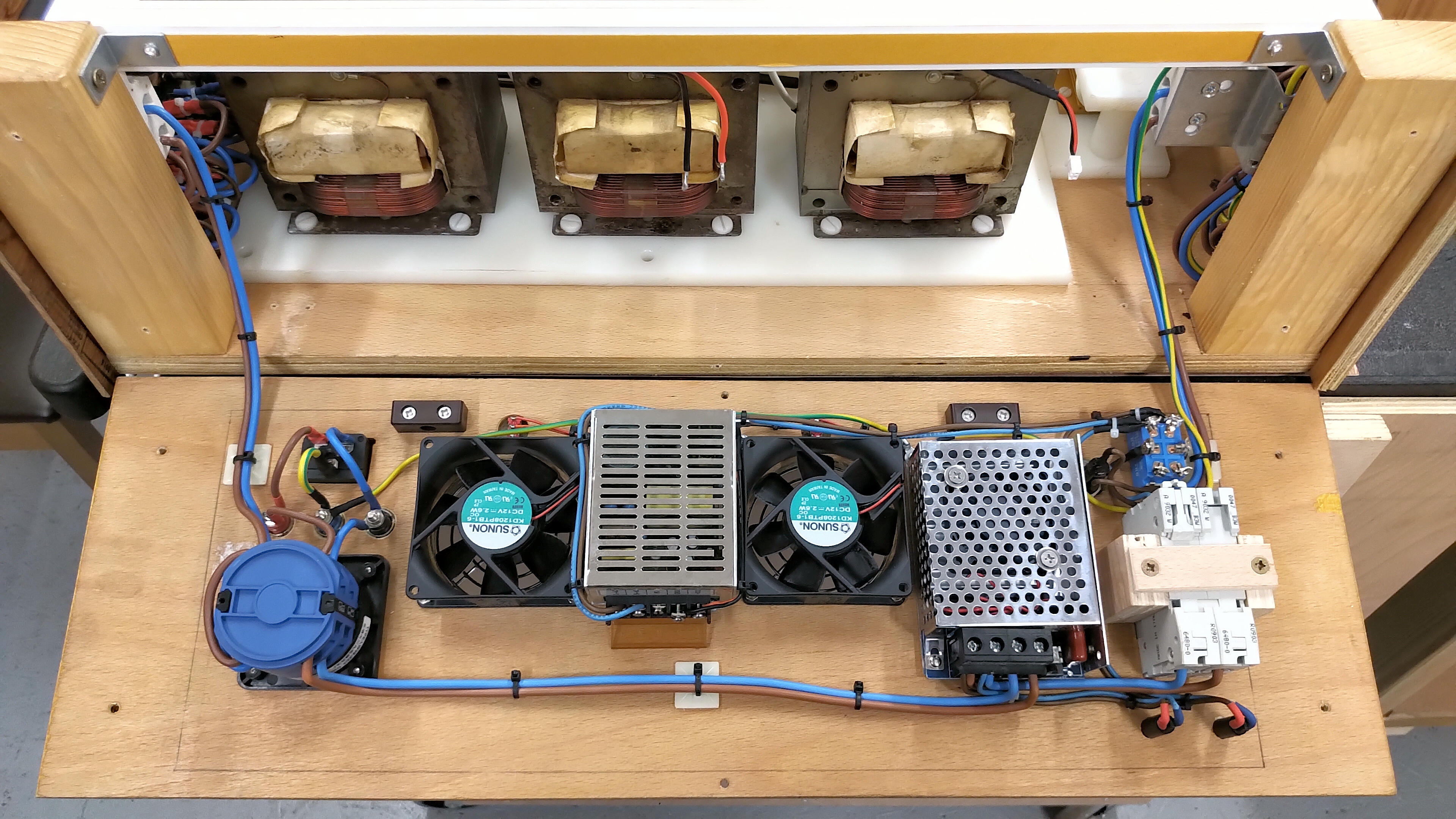
2. A high power 5kW plate supply using three 1.8kVA industrial microwave oven transformers, that can be configured in a variety of parallel and series arrangements to provide plate supplies including 2kV @ 2.3A, 4kV @ 0.8A, and up to 6kV @ 0.8A. A high voltage 40kV 6A bridge rectifier is incorporated into the design, along with a 12kV rapid discharge unit for safely discharging tank capacitors in the driven circuit. Also internally installed is a 4uF 6kV level shifter to increase the output up to 12kV @ 300mA and 15kV @ 150mA, which is suitable to drive medium power thyratron tubes, such as the 5C22 for pulse and impulse discharge experiments, as well as displacement of electric power experiments. I will be covering the design, construction and operation of this supply in a subsequent post.
3. A dual 833C RF Power Triode tube board with graphite plates and with continuous axial cooling, driven at 4kV plate supply and with a total usable output power of ~ 3.0kW @ 2Mc, and the heater drive is 10V @ 20A AC for both tubes. The graphite plates of the C variant of the 833 tube improve significantly the top-end performance of this tube board by reducing plate to grid flash-over under high-power or poorly matched output conditions. Suitable for displacement and transference of electric power experiments, Tesla’s radiant energy and matter experiments, and including plasma, induction generator, and discharge phenomena.
4. A quad 811A RF Power Triode tube board with continuous axial cooling, driven at 1.2kV plate supply and with a useable output power of ~ 1kW @ 2Mc, and the heater drive is 6.3V @ 16A for all four tubes. This is a very versatile and flexible day-to-day workhorse with lower plate supply requirements, and facilitates a wide range of Tesla experiments as already demonstrated on my website using power up to 1kW.
5. A dual 4-400A RF Power Tetrode tube board with continuous axial cooling, and which is particularly good for high-fidelity musical Tesla coils, and linear amplifier type experiments where modulation and signal purity combined with good output power are required.
6. A dual 810C Power Triode tube board with graphite plates and continuous axial cooling, and which is particularly good for driving lower frequency Tesla coils in the hundreds of kilocycle frequency range, and with good power modulation and signal linearity.
The design, construction and operation of these tube boards will be covered in more detail in subsequent posts, and also operation of the complete tube power supply system as part of experiments yet to be presented on the website. So let us now get on with the tube power supply – heater, grid & screen unit with a video overview of its design, construction, and operation, and including driving a basic experiment using a single cylindrical Tesla coil with a single wire load. The video also demonstrates the use of both the dual 833C and quad 811A tube boards, here used as tuned plate class-C Armstrong oscillators, deriving linear feedback directly from the secondary coil oscillation, and primary circuit tuned to drive the cylindrical Tesla coil at the upper and lower parallel resonant frequencies.
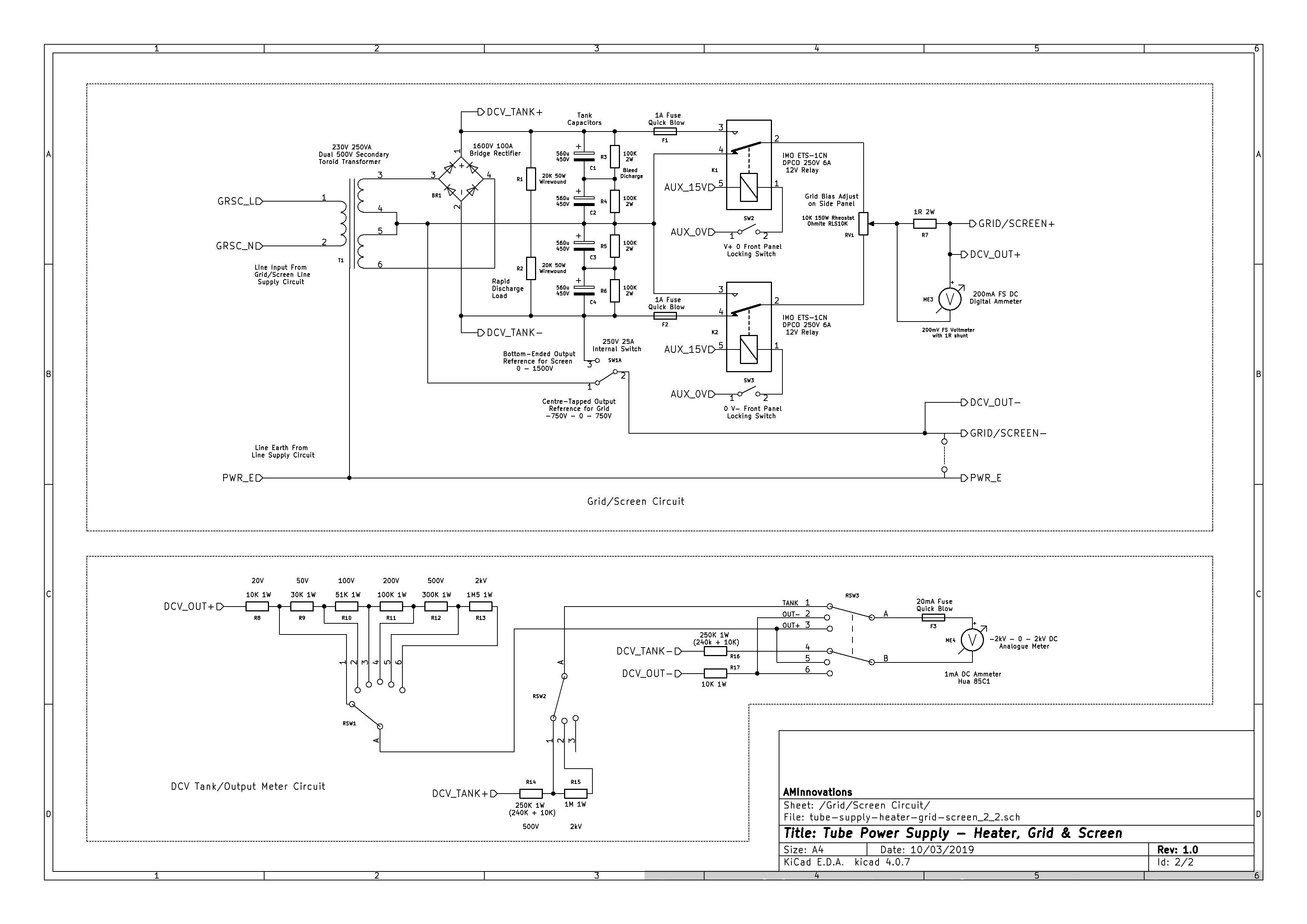
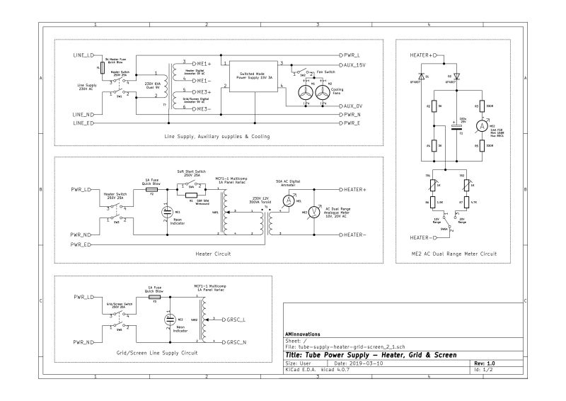
The circuit diagrams for the TPS-HGS are shown in Figures 2 below. To view the high-resolution versions click here on Fig 1.1 or Fig1.2.
Fig. 1.1 Tube power supply schematic showing the main line supply circuit, auxiliary supplies, the complete heater circuit, and the line supply for the grid/screen circuit.
Fig. 1.2 The tube supply schematic showing the grid/screen circuit, and the tank/output meter circuit.
The principle of operation for the heater supply unit is as follows. This supply provides a high current low voltage output to drive the filaments in the tube board when connected in series or parallel arrangements. The internal resistance of the vacuum tube filaments determine the supply requirements without any additional regulation at the supply end. To this effect a 12V 300VA transformer can be adjusted using a variac to correctly bias the requirements of the tube board both in voltage and current. The power rating of the transformer was selected to adequately cover the various tube boards being used, and is capable of a maximum of 12.6V @ 25A. Open circuit the supply provides 15.9V which reduces with increased load, and to the correct filament voltage and current when adjusted by the variac.
A soft-start switch is incorporated to switch a resistive load 50Ω 50W into the primary circuit of the transformer, which reduces the potential across the primary, and hence reduces the secondary output. When vacuum tubes are cold the filament resistance is generally much lower than when in normal operation, and the initial in-rush of current when power is first applied to the filament circuit can easily exceed the maximum safe ratings, which can lead to significantly reduced filament lifetime and premature failure of the filaments in one or more tubes. The ac voltage and current supplied by the heater supply is monitored using an analogue true rms circuit through a DC 1mA ammeter, and a digital 50A AC ammeter based on the potential difference across a 75mΩ series resistance in the output circuit.
The digital ammeter is most effective for setting accurate bias current prior to RF circuit operation. The outputs of the heater circuit are arranged flexibly on the back panel to allow rapid and configurable connection to the tube boards, and including the ability to float the filament supply above the line supply earth. Disconnecting the heater supply from the line earth allows the vacuum tube to be cathode switched, modulated, or “pulsed”, and for the tube board to be referenced to a different “ground” e.g. a dedicated RF ground, or plate supply with high voltage biased negative, (useful for extreme high-voltage thyratron supplies).
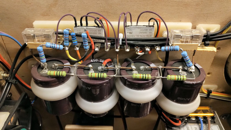
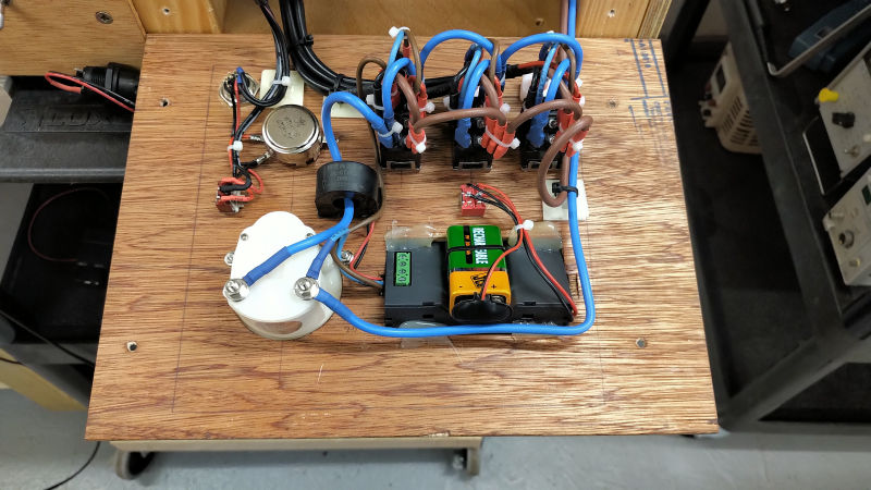
The principle of operation for the grid/screen bias unit is as follows. This supply provides a stable unregulated output bias based on the voltage accumulated in a tank circuit, and which can be finely controlled by a high power potential divider to the output. A high-voltage transformer with dual secondary coils rated at 500V each with a total power output of 250VA is adjusted using a variac on its primary circuit. This gives a variable output voltage of ±500VRMS @ 200mA when negative reference is at the centre tap, or 1000VRMS @ 200mA when negative reference is at the bottom-end of the lower secondary coil. The output of the high-voltage transformer is bridge rectified and then accumulated on a tank capacitor circuit consisting of 4 x 560µF 450V capacitors in series. Bleed resistors and a high-power parallel load resistance are provided for rapid discharge of the tank when switched off. The tank is intended to provide a stable DC supply with very low output ripple up to 200mA for grid and screen bias purposes.
To facilitate very fine adjustments in grid bias, which is often very necessary to establish the best operating point for a tube amplifier or oscillator, the output of the tank circuit is fed through a 150W 10kΩ rheostat, which provides continuous linear adjustment of the output across the entire range of the tank voltage. This allows for initial setup of the tube board prior to application of the plate supply, and then variable bias tuning during operation of the experiment. As the bias output is unregulated changes to the experimental conditions will effect required changes to the grid bias and this can be safely and readily applied through the grid bias rheostat. The final result is a very flexible supply that can accommodate a wide range of different tubes and operating conditions. Rapid adjustment of these parameters in a research and development context greatly reduces experimental setup and adjustment time, and facilitates easy tuning to find the most optimum point of operation.
The rheostat fine control is fed from the tank capacitors via two changeover high-voltage relays that switch the output between the upper and lower secondary coils, or across both coils. This allows the output range to be more precisely and safely controlled by selecting just a negative output range, a positive output range, or the entire tank range. This has benefit for example when biasing a tube board in grounded cathode for linear amplifier application. Here the grid bias for a class C linear amplifier is usually in the negative range, so to minimise power dissipation in the grid adjust rheostat, and to ensure that the bias cannot drift into positive voltage with higher risk of tube damage, the output relays are configured to connect only the negative section of the tank circuit across the grid adjust rheostat and hence to the output.
Measurement of DC tank voltage, and output bias voltage is accomplished by a switched series resistance which scales the current into an ammeter up to 1mA. For greater accuracy and scale size the analogue meter is switched either to measure a negative bias potential, or a positive bias potential, by switched reversal of the measurement current through the meter. This series resistance method gives a very good dynamic range of measurement with ranges between 20V DC FSD, and 2kV DC FSD. The process of operating the grid/screen supply requires that the tank voltage first be set to a value higher than is required for the output bias, and then the output bias set through the fine control of the grid adjust.
The switching between these measurements is quickly and easily facilitated by the rotary controls on the front panel of the instrument. The rotary switches are plastic spindle types, which also provide excellent isolation during operation from internal high voltage. It should also be noted that the switched series resistance also has part of that resistance chain in the negative terminal of the output e.g. R14, R15, R16, R17. These resistors prevent current surges between the various output circuits during switching of the measurement ranges, and also inadvertent changes to the setting of the tank output relays when the tank circuit is not discharged. This is particularly important at high tank voltages where switching could otherwise result in large surge currents and destruction of the relays, and other switching components. I discovered this one during inital supply tests, and needed to change both relays and a rotary switch that had burned and fused contacts from a surge at maximum tank setting of 1500V!
Measurement of DC output current is by digital ammeter with 200mA FS. The digital meter is a 200mV FS DC meter which has a 1Ω 2W shunt resistor at the output of the grid adjust rheostat. As for the heater supply, the digital readout facilitates accurate bias adjustment and setup prior to operation of the tube board at RF frequencies. Overall the two supply units are simple in design and construction, and compact and cost effective in materials and components, but lead to a very wide range of operating characteristics, which can be quickly and easily adjusted by a skilled operator during the experimental process.
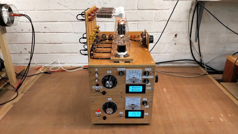
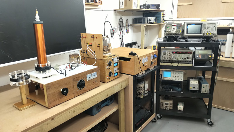
Figures 2 below show the complete unit with both the dual 833C and quad 811A tube boards installed. The pictures illustrate the compact yet powerful design, and particularly the space saving footprint on the bench. When combined with the 5kW high-power plate supply, the two together form a very versatile and robust tube power supply suitable for a very wide range of Tesla and high-voltage research experiments including, displacement and transference of electric power, Telluric transmission of power, radiant energy and matter, modulated and high-fidelity waveforms, and plasma and discharge phenomena. The same plate supply combined with a specialised 5C22 thyratron board and pulse trigger unit is well suited to displacement of electric power, pulse, impulse, and unidirectional discharge phenomena.
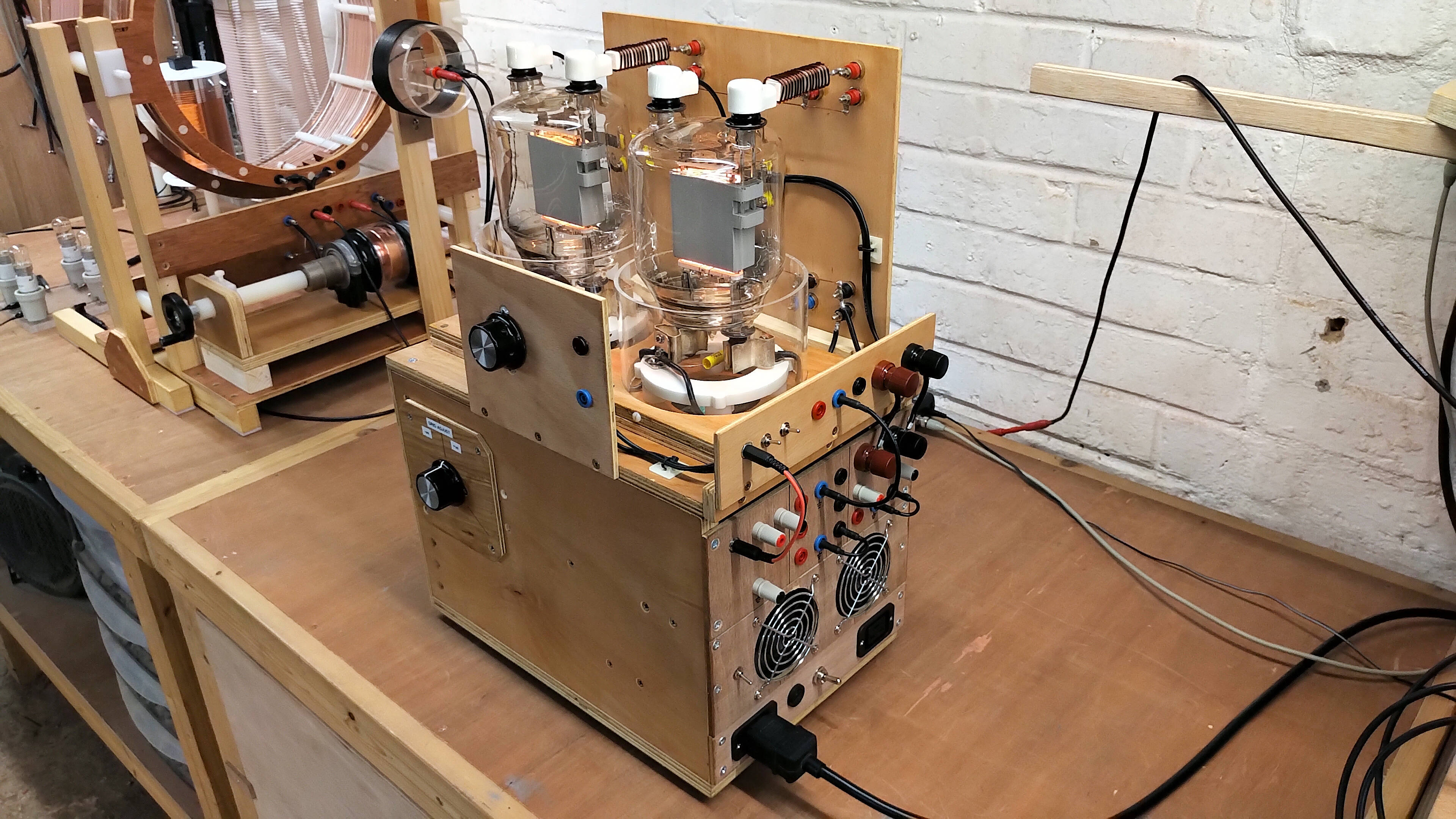
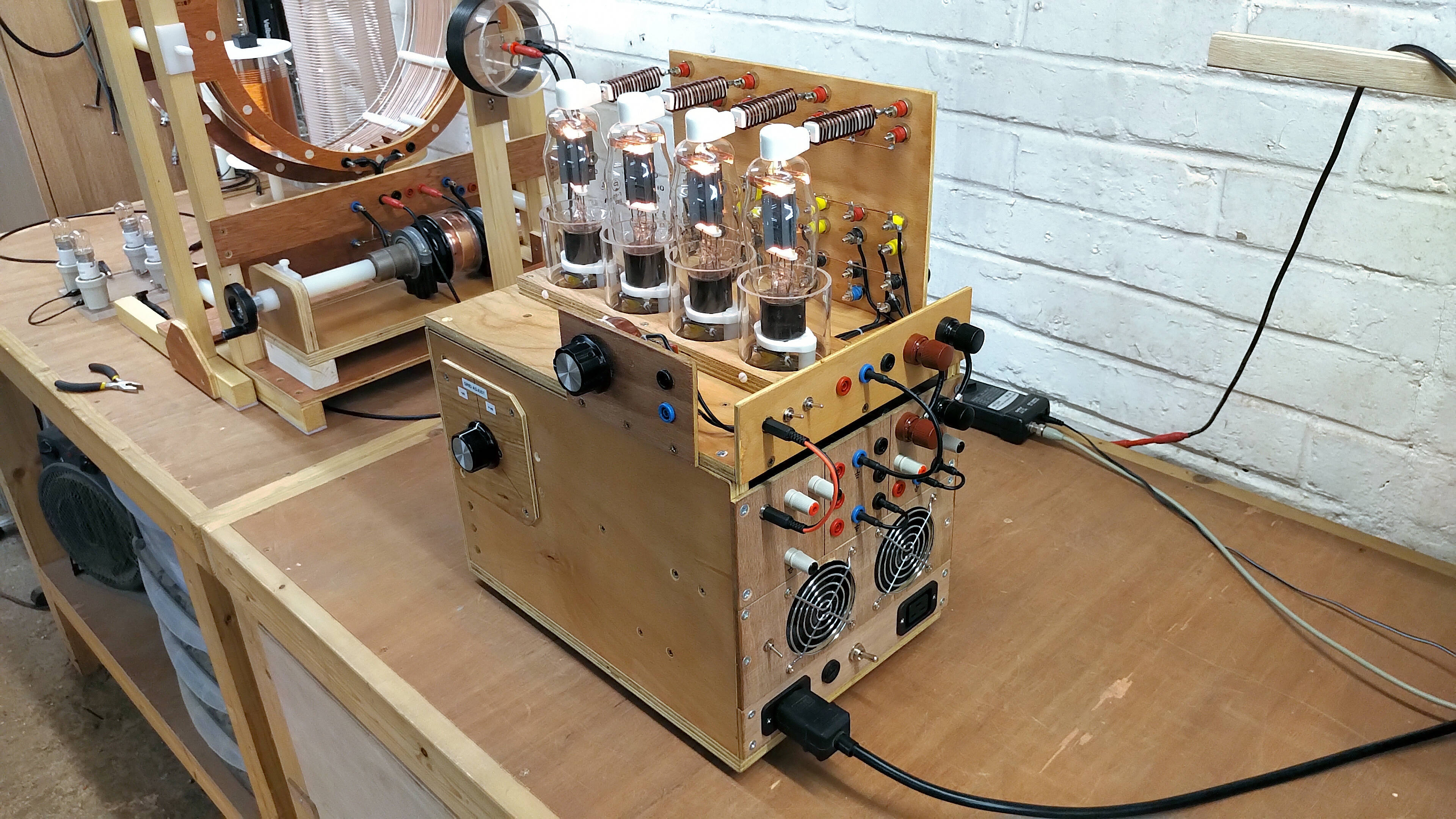
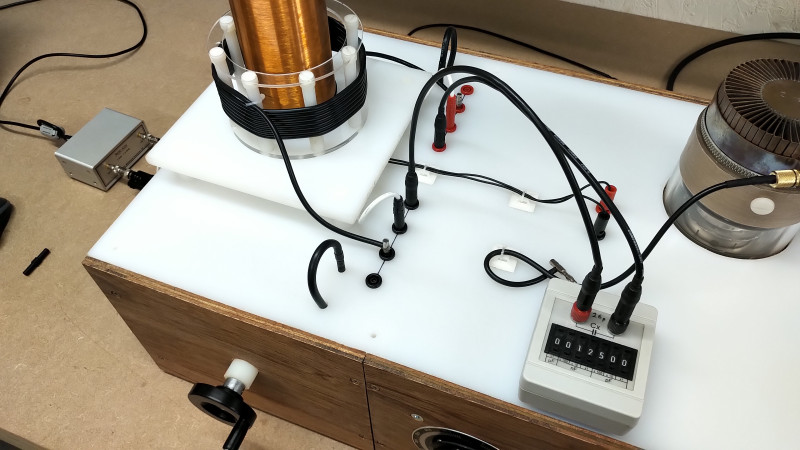
Fig. 2.1 The tube supply with the dual 833C tube board. The heater circuit is active and set to 10V AC @ 20A which fully powers the heater filaments in the two tubes. The Grid supply is not being used here.
Fig. 2.2 The dual 833C tube board has adjustment on the side for grid bias when used as a tuned plate Armstrong series feedback oscillator.
Fig. 2.3 The tube board is connected to the supply at the rear for the heater power, in this case grid oscillator grounding, and the low-voltage supply to power the cooling fans.
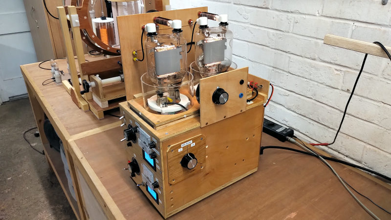
Fig. 2.4 Here the quad 811A tube board is installed and warmed up before operation. Each tube requires a filament voltage of 6.3V @ 4A. The heater supply is set to 6.3V @ 16A for four tubes in parallel.
Fig. 2.5 As before the 811A tube board has grid bias adjust when being used an Armstrong oscillator. Here the grid bias rheostat is much smaller than before as the grid dissipation is lower for these tubes.
Fig. 2.6 Connection of the 811A tube board to the supply is the same as for the dual 833C board, and shows the ease with which a different configuration can be setup and operated in the research environment.
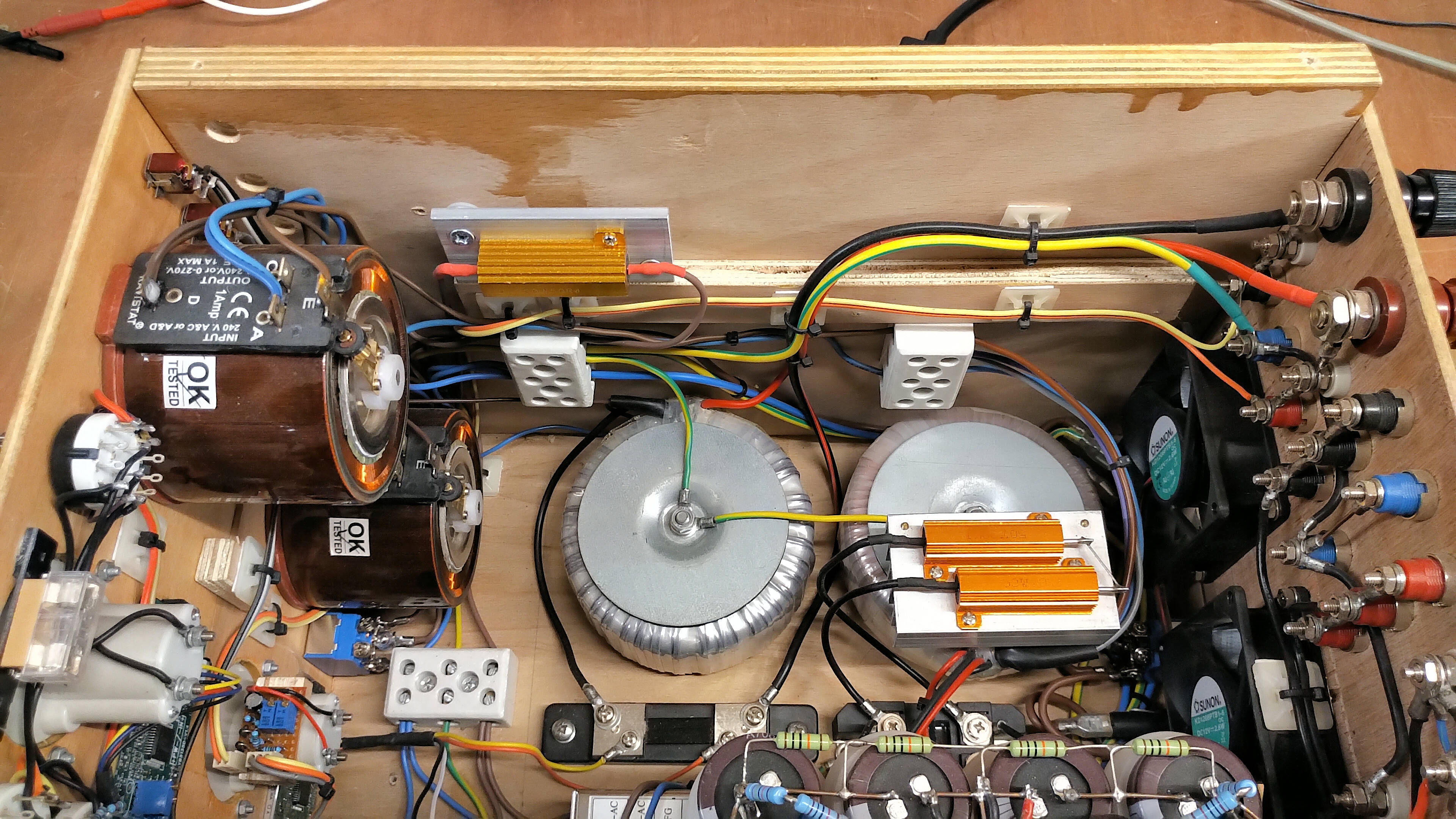
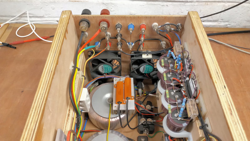
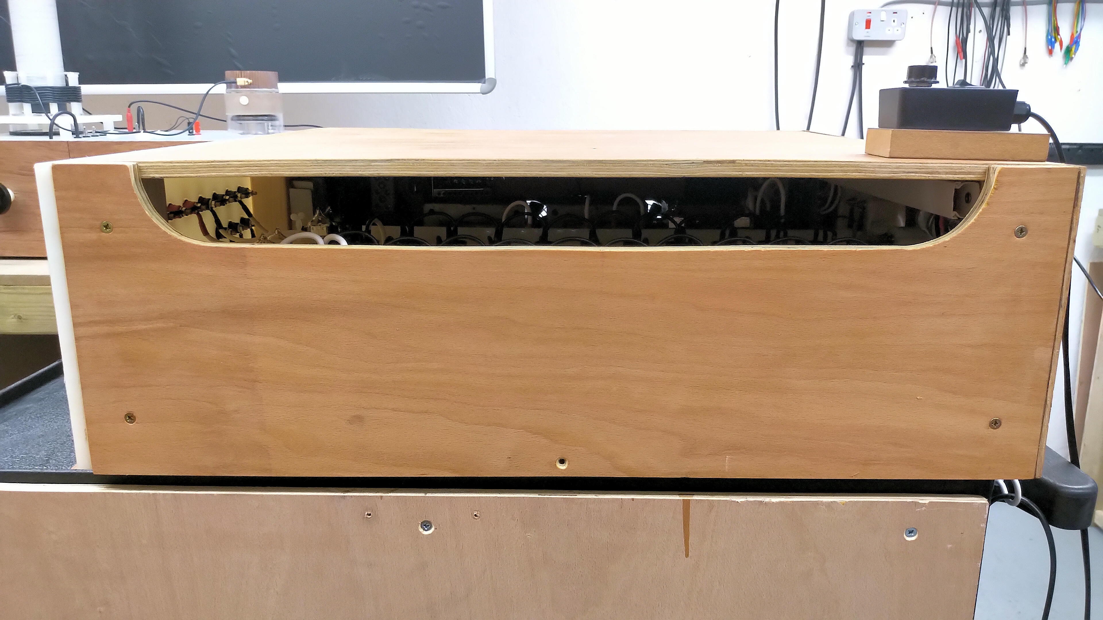
Figures 3 below show the internal layout and construction of the complete heater, grid & screen tube supply. The entire unit is housed in an oil varnished plywood housing, with consideration for cooling, correct line earthing of the appropriate components, internal safety of the high-voltage components and regions, and the external safety of the operator with the various controls when adjusted during the experimental process. As discussed on the video, the choice of a wooden enclosure faciltates easy fabrication and construction, with reasonable thermal properties when fan-cooled, and reasonable external isolation from high-voltage components and regions.
The wooden enclosure does not facilitate grounding and earth connection of certain components, which requires more considered wiring and interconnection of line earth around the internal layout. The wooden enclosure provides no EMI protection either externally to other objects in the facinity, or internally from electric and dielectric fields of induction around the experiment. In a research and development environment in an industrial and isolated setting this is considered acceptable given the often short operation time periods, and minimum interference to surrounding infrastructure.
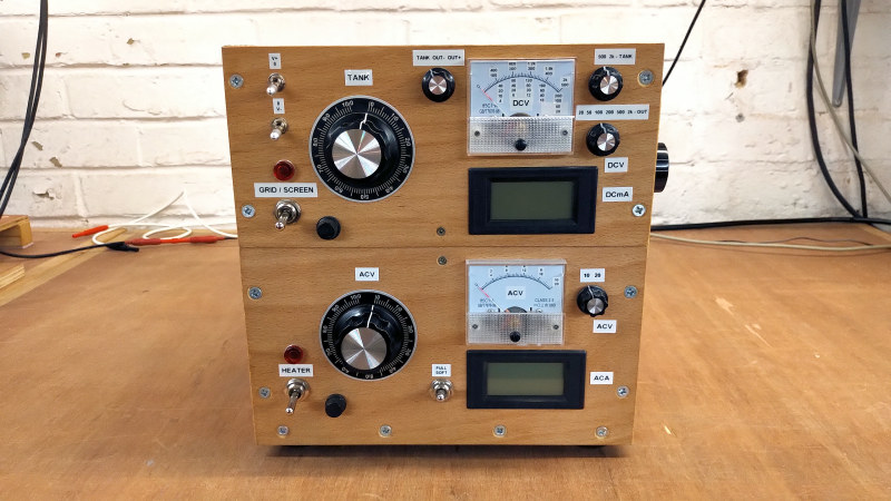
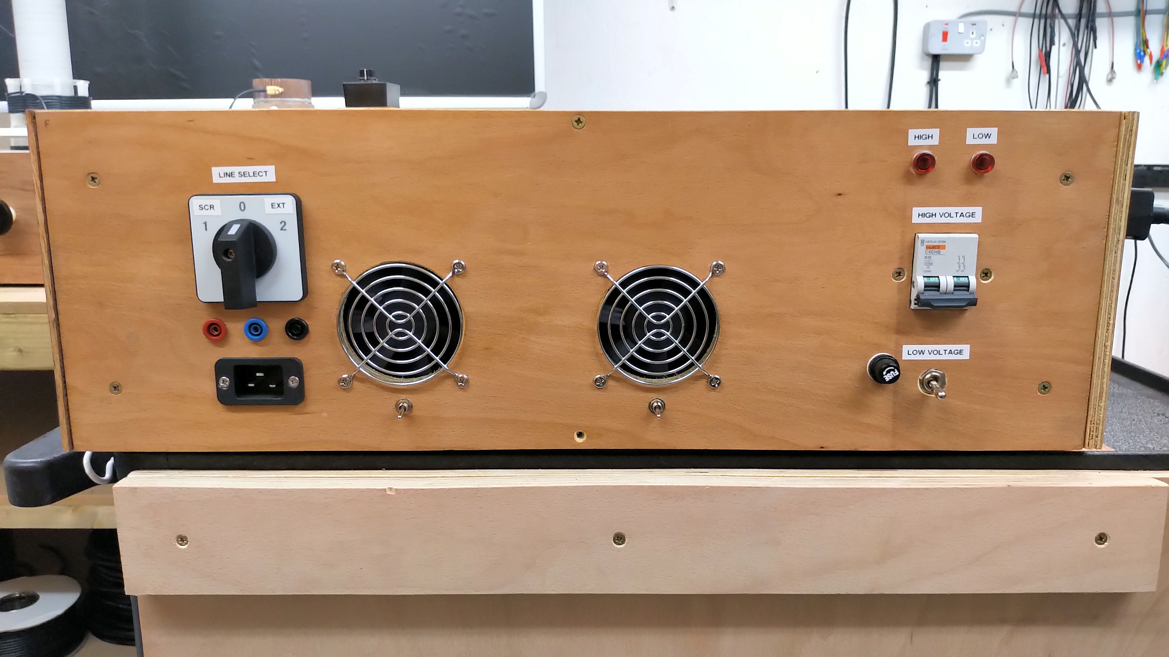
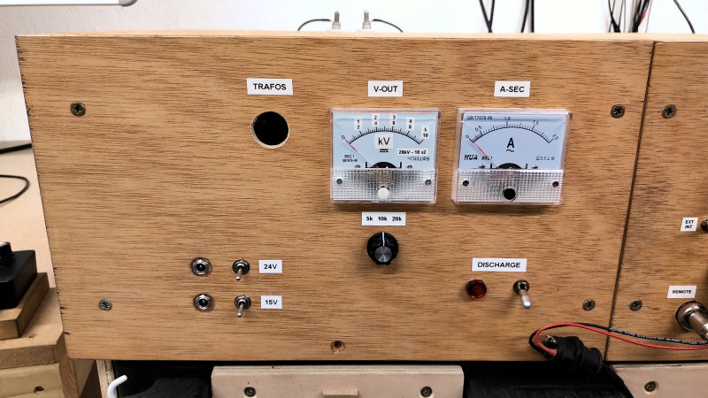
Fig. 3.1 The front panel of the tube supply has independent heater and grid/screen supplies. Voltage and current output in each supply is measured using analogue and digital meters. The system is designed to be simple, versatile, and quick to adjust and configure.
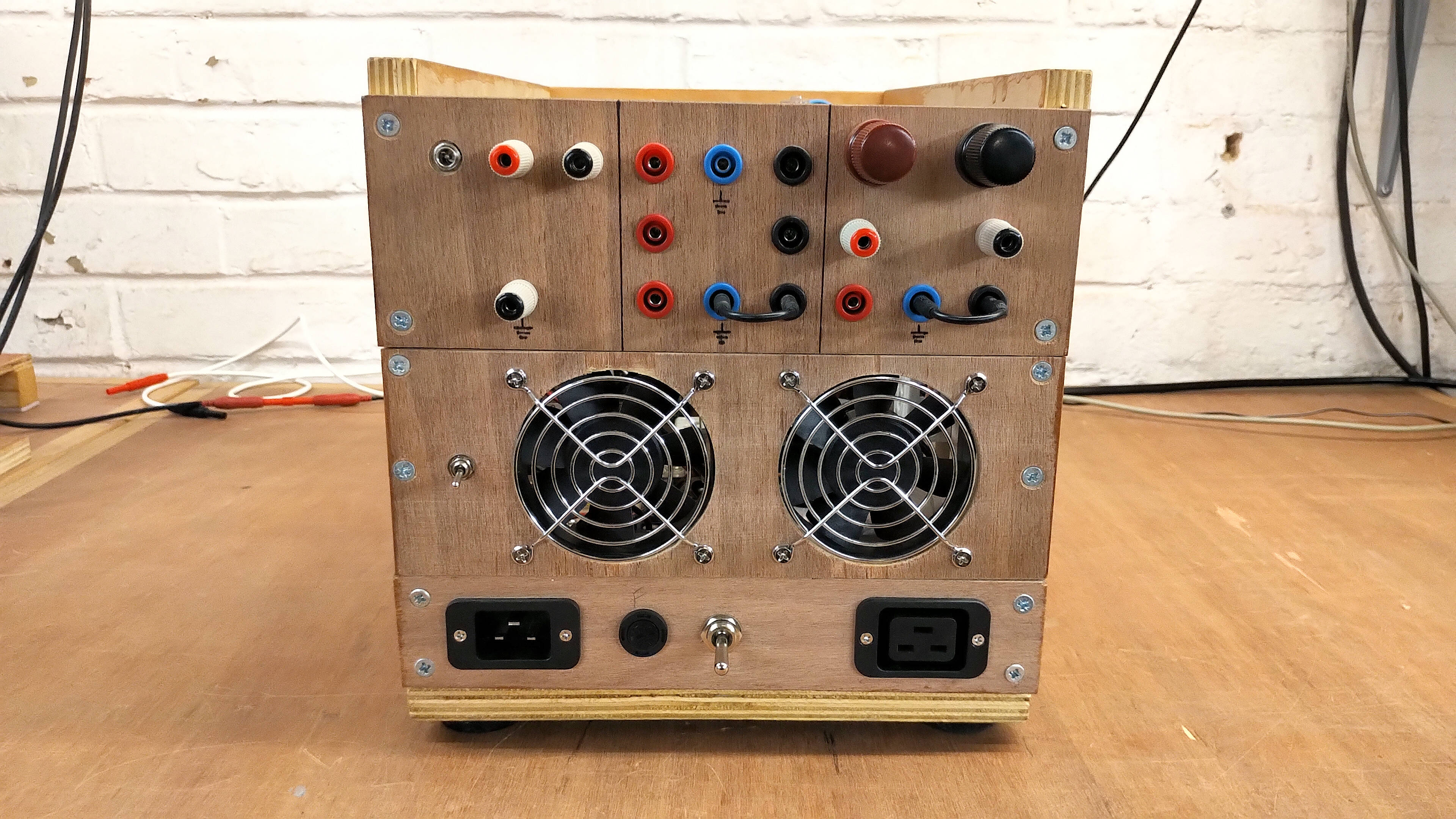
Fig. 3.2 The rear panel has the ine supply input, master switch and fuse, along with the cooling panel, and the output panel. The output panel has sections for lov voltage 15V, grid bias, and heater supply .
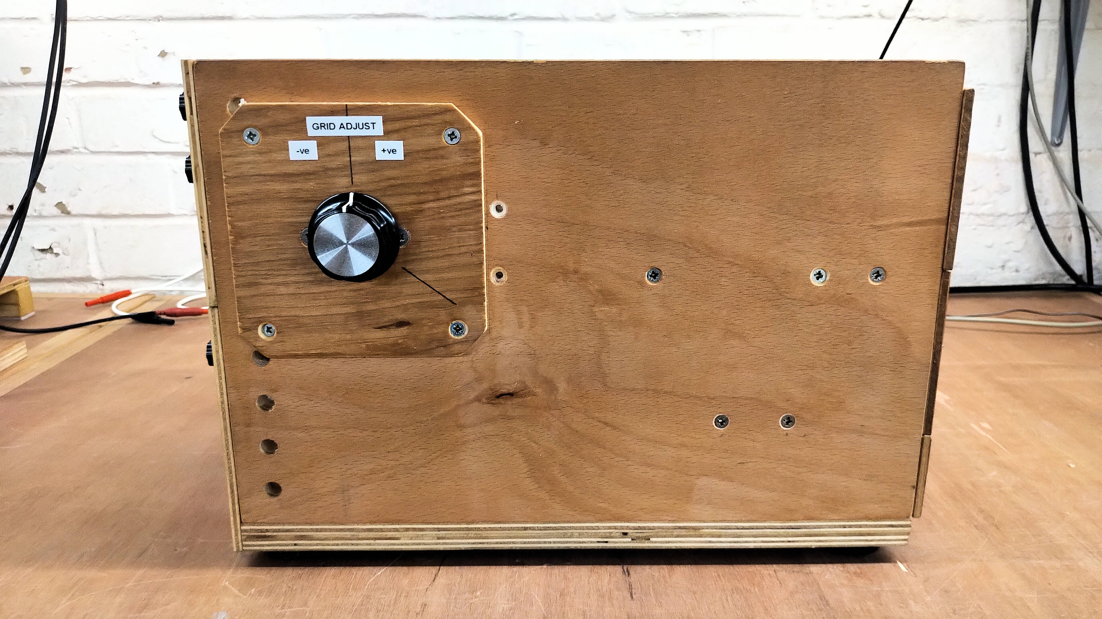
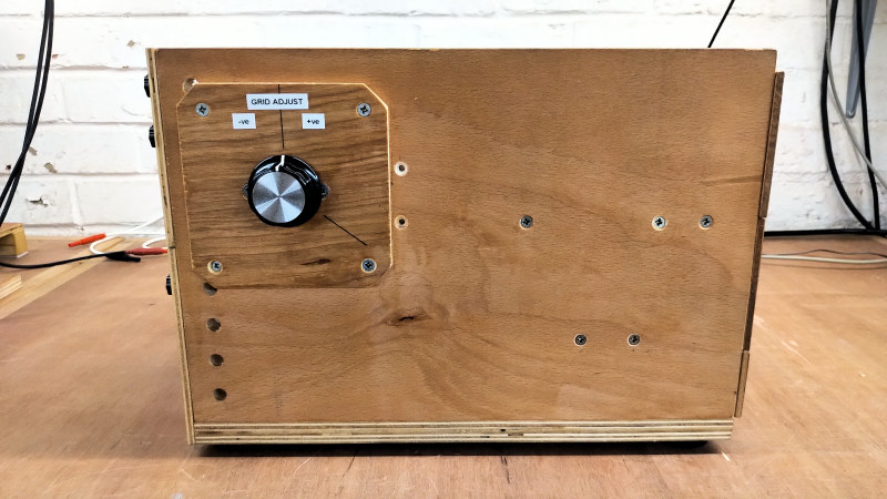
Fig. 3.3 The right side panel has the grid bias adjust rheostat, which allows fine control of the grid bias over the entire tank range from positive to negative, and fine screen bias adjust in the positive range. Cooling holes are drilled at the front on both sides.
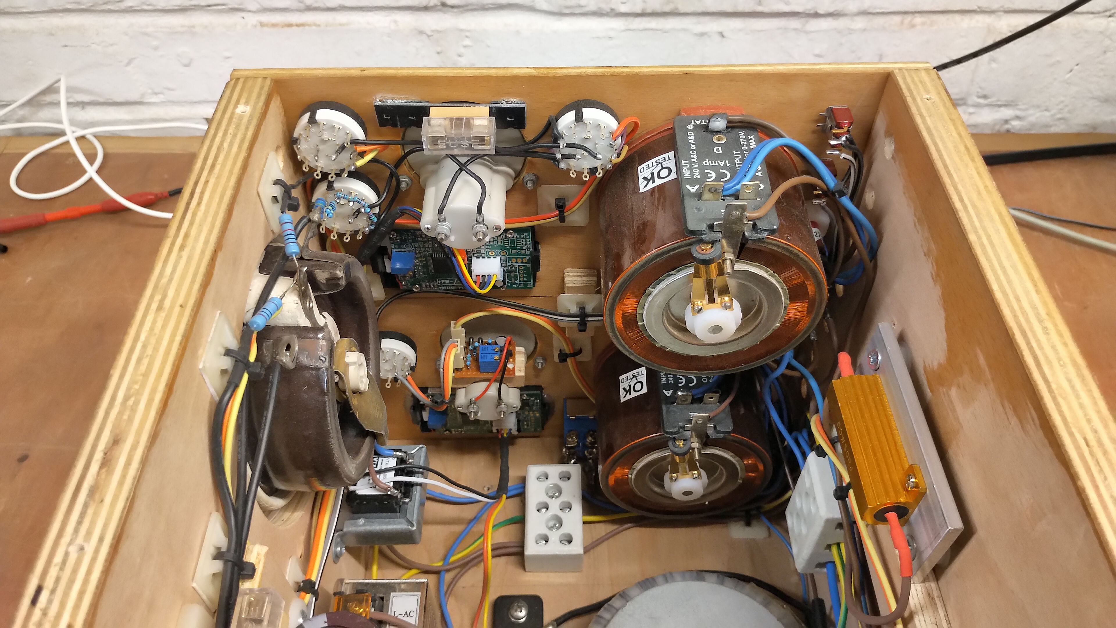
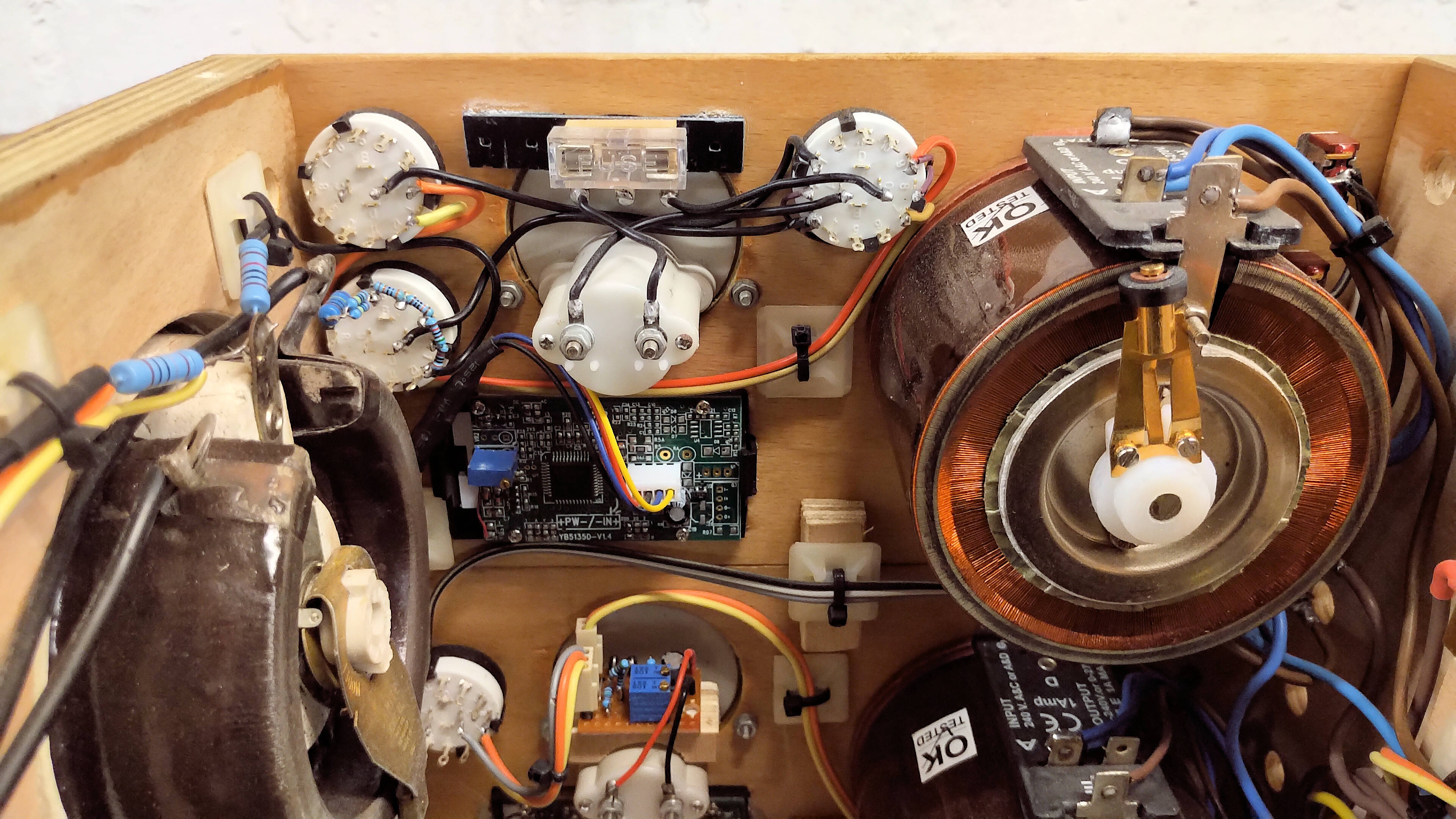
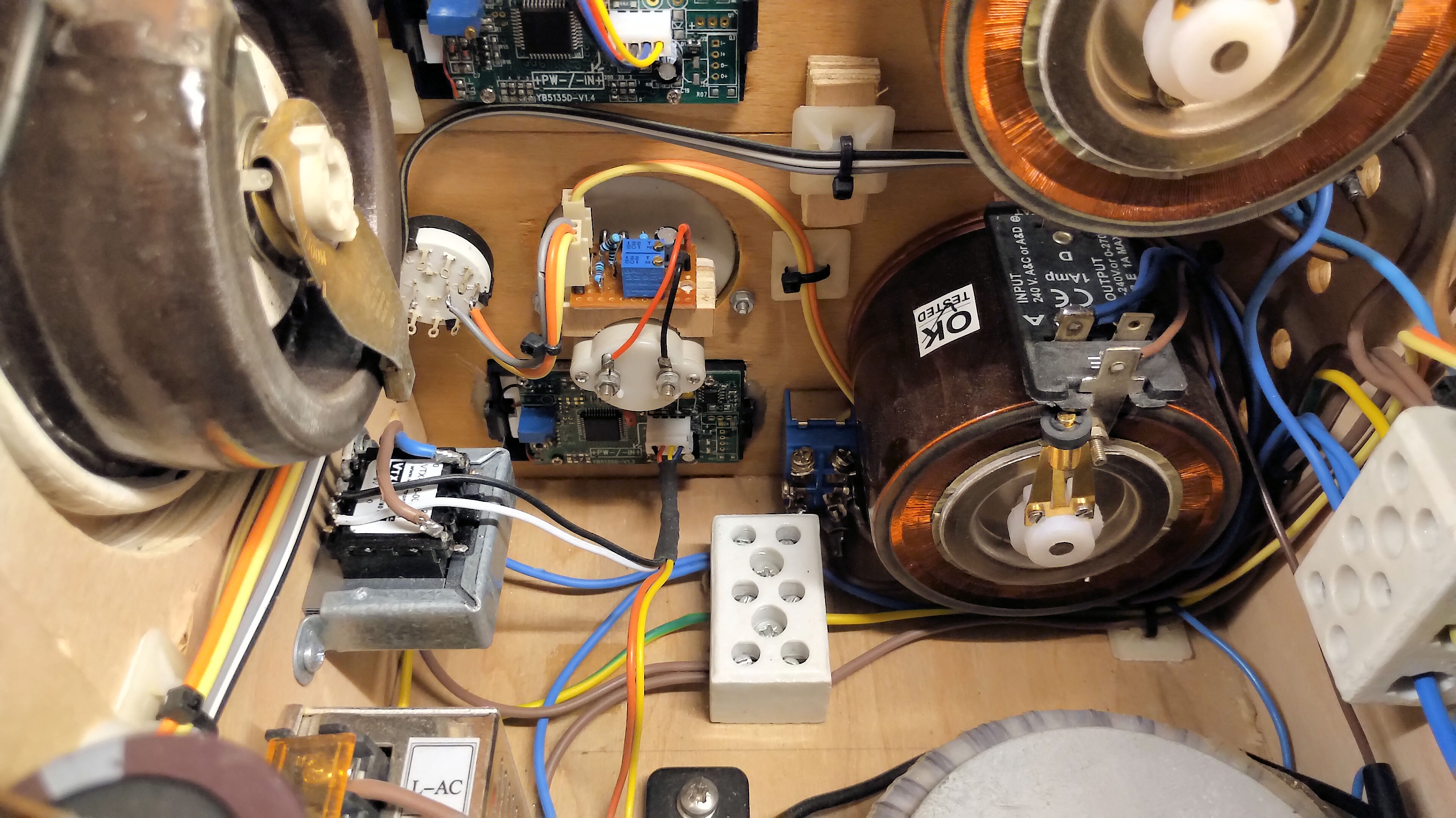
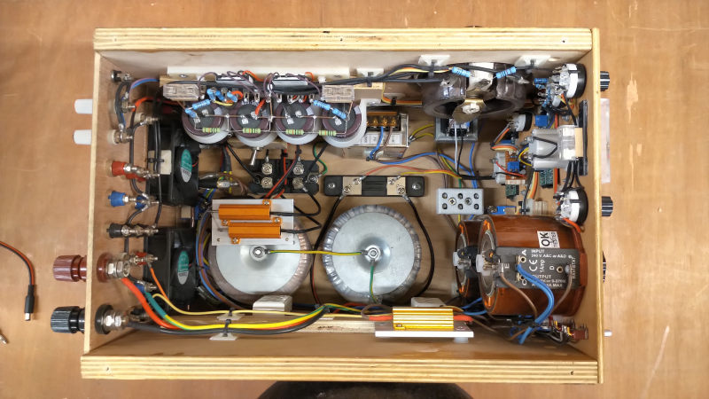
Fig. 3.4 An overall view of the inside of the tube supply, showing that even a relatively simple design requires careful layout, wiring, and economic use of space.
Fig. 3.5 The right inner side showing mostly the tank circuit for grid bias, and the fine output adjust rheostat. Below the tank circuit is the internal negative output reference switch to change between grid and screen bias reference.
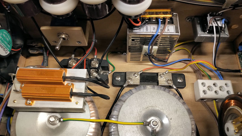
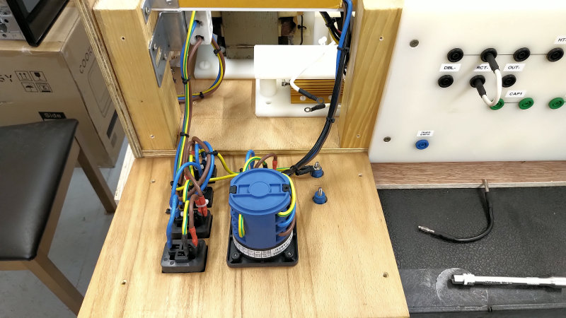
Fig. 3.6 The inside rear panel showing the output connections and cooling panel, and in front of this the grid circuit toroidal transformer with heatsink mounted rapid tank discharge resistive load.
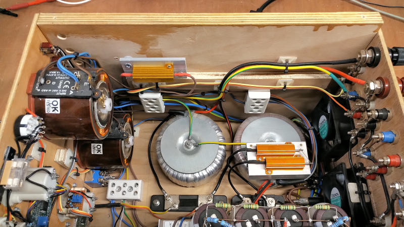
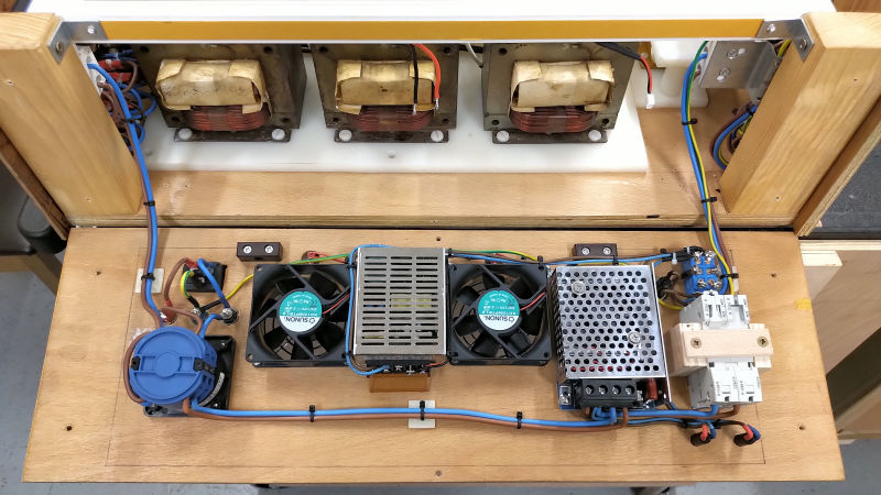
Fig. 3.7 The inner left side showing the two toroidal transformers for the heater and grid, and the variacs that control the line input to both of the main supply sections. The left side also has most of the line supply wiring and earth wiring for those components that need earthing.
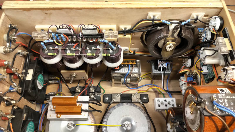
Fig. 3.8 The front inner panel showing again the variacs, and the switching and metering circuits that allow control of both the heater and grid/screen sections. The soft-start resistive load is heat-sinked and mounted in the bottom right of the picture.
Fig. 3.9 A close-up of the inner front panel upper grid/screen control section.
Fig. 3.10 A close-up of the inner front panel lower heater control section.
Fig. 3.11 A close-up of the inner right hand panel tank circuit, including the bias output relays to control the active output range.
Fig. 3.12 A close-up of the right side panel below the tank circuit showing the negative terminal reference switch, the 15V switched mode supply, dual 9V meter transformer, and the toroids, rectifier and tank discharge load.
It can be seen from figures 3 that the overall layout and construction is relatively straightforward. Care with proper positioning and wiring of the high voltage components is very important, particularly in spacing of contacts, the wire type used to connect the high voltage components, and isolation from the user controls on the front-panel. Otherwise a flexible design is possible from a simple circuit, is easy to diagnose and fix if and when a problem occurs, and facilitates a very wide range of experimental conditions that can be adapted, adjusted, and tuned quickly in a research and development prototype setting.
The next parts in this tube power supply series will cover the plate supply, and the individual tube board designs and circuit configurations.
Click here to continue to the next part, looking at Tube Power Supply – High Voltage & Plate.
1. A & P Electronic Media, AMInnovations by Adrian Marsh, 2019, EMediaPress
2. Dollard, E. and Energetic Forum Members, Energetic Forum, 2008 onwards.
In this second post on the Tube Power Supply series I present a complete design and implementation of a high voltage (HV) unit suitable for use as a high-power plate supply, and also as a general purpose high-tension source for a wide range of experiments in electricity. I use this unit extensively in my own day-to-day research for experiments in the displacement and transference of electric power. The 5kW high voltage and plate supply is based around three heavy-duty industrial 1.8kVA microwave oven transformers which can easily be inter-connected in a range of different parallel and series configurations. The transformers can be easily combined with different output stages including a bridge rectifier, level shifter (doubler), and a high voltage discharge unit, which are all incorporated into the complete housing of the supply. The complete high voltage supply is housed in a traditional varnished wooden enclosure and is designed to fit together with the other supply components in the tube power supply series.
Note: A high voltage supply is capable of delivering voltages and currents, even at lower powers, that are instantly lethal, and that any design and operation of a high voltage unit should be undertaken with great care by a trained and experienced individual. The high-voltage supply presented in this post is intended for high-power electricity research experiments undertaken by trained and experienced operators only. The different transformer configurations combined with the different output stages make for a very versatile, robust, and adaptable high voltage and plate supply with a fully loaded output ranging from 2.1kVRMS @ ~ 2.3A all the way up to 15kVRMS @ ~ 150mA. This very wide output range currently accommodates all of the tube amplifiers, oscillators, and impulse generators that I use in my own research, including the following examples that are used in experiments presented, or yet to be presented, on this website:
1. A basic parallel connected quad 811A linear amplifier or Hartley power oscillator, using 1.2kV plate supply and producing about 1kW of sustained output power at frequencies up to ~4Mc.
2. A parallel connected dual 833C class-C Armstrong oscillator using a 4kV plate supply and producing up to 2.5kW of sustained output power at frequencies up to ~4.5Mc.
3. A single GU5B class-C Armstrong oscillator using a 4-5kV plate supply and producing up to 2kW of sustained output power up to ~3Mc, or even using a 9kV plate supply when used in pulsed-mode with a low duty cycle.
4. A dual push-pull connected 4-400A linear amplifier using 4kV plate supply and producing up to 1kW of power up to ~5Mc.
5. A dual 5C22 hydrogen thyratron pulse generator, with an anode supply up to 15kV.
Figure 1 below shows a summary table of the main setup configurations that can be arranged with the presented power supply, and the nominal outputs that can be achieved using that configuration, and with the various indicated output stages. These performance characteristics are presented as a guide to the configuration and usage of this high voltage supply, and may vary according to the type of load or generator being driven, the impedance match conditions between the supply and the generator and experiment, and also the type and condition of the transformers used in the supply build.
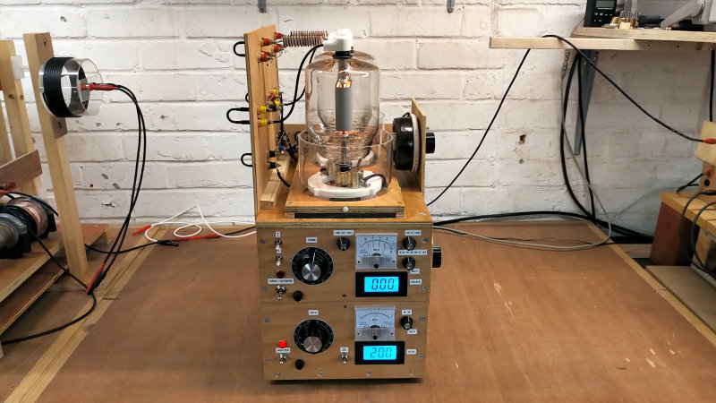
The following video takes a detailed look at the high voltage plate supply, its design, development, and implementation, how to configure and setup the required operation mode, the different output stages, the various safety requirements during its operation, and concluding with a demonstration of its operation during experiments in the Wheelwork of Nature series, when used with the single GU5B class-C Armstrong oscillator generator.
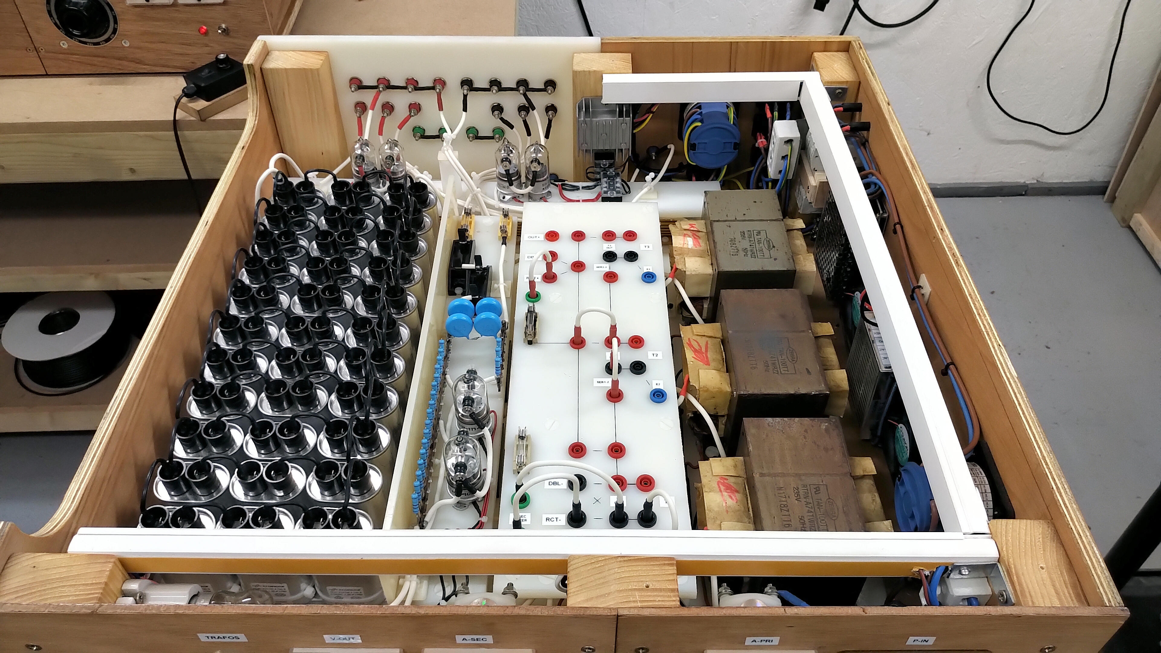
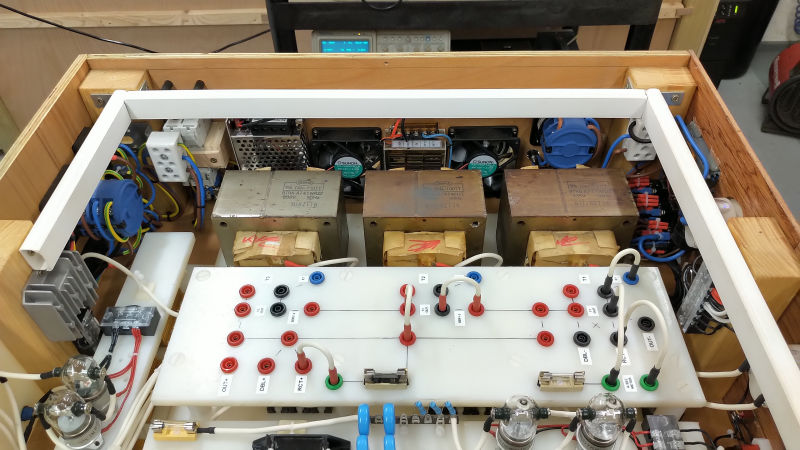
Figures 2 below show the high voltage and plate supply in detail both from the exterior panels and sides, through to the internal modular boards, layout, and construction.
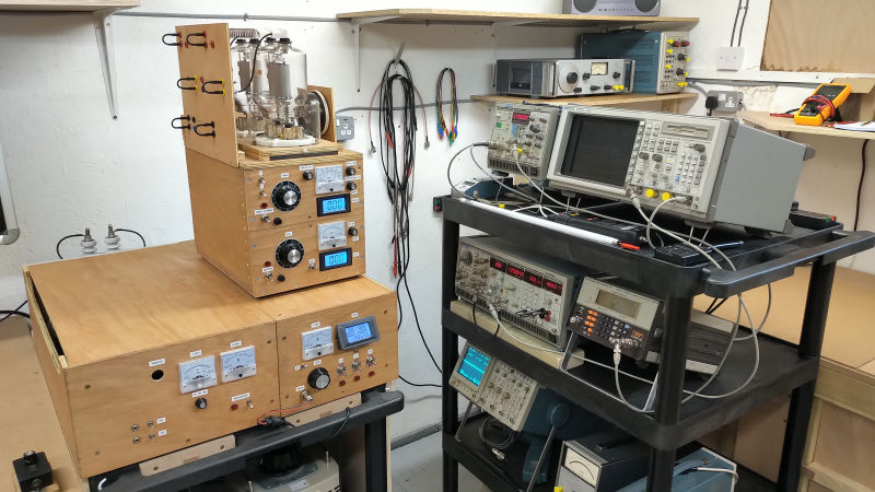
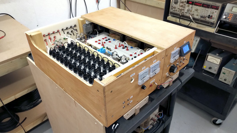
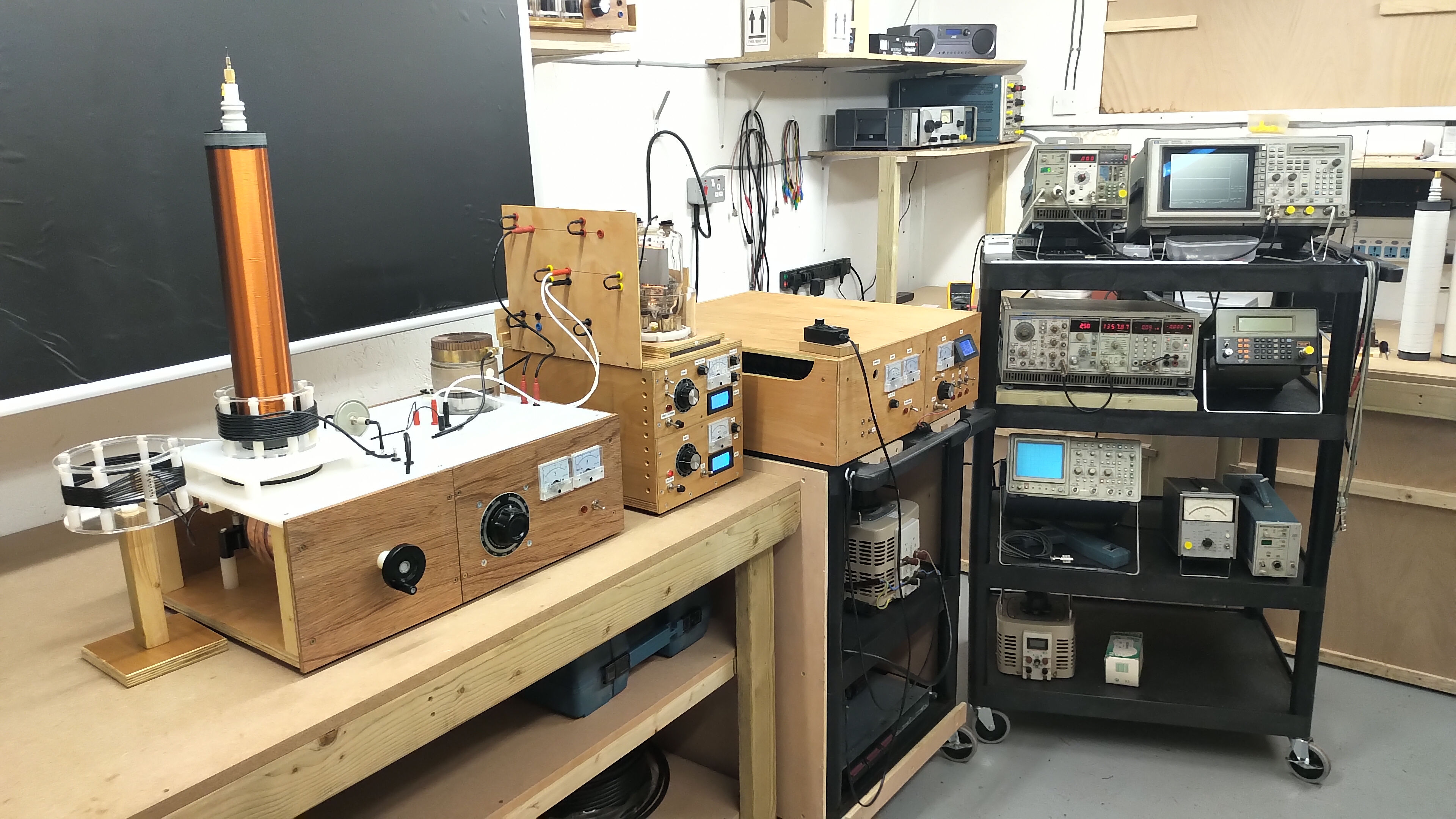
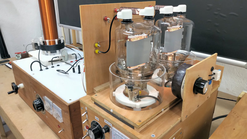
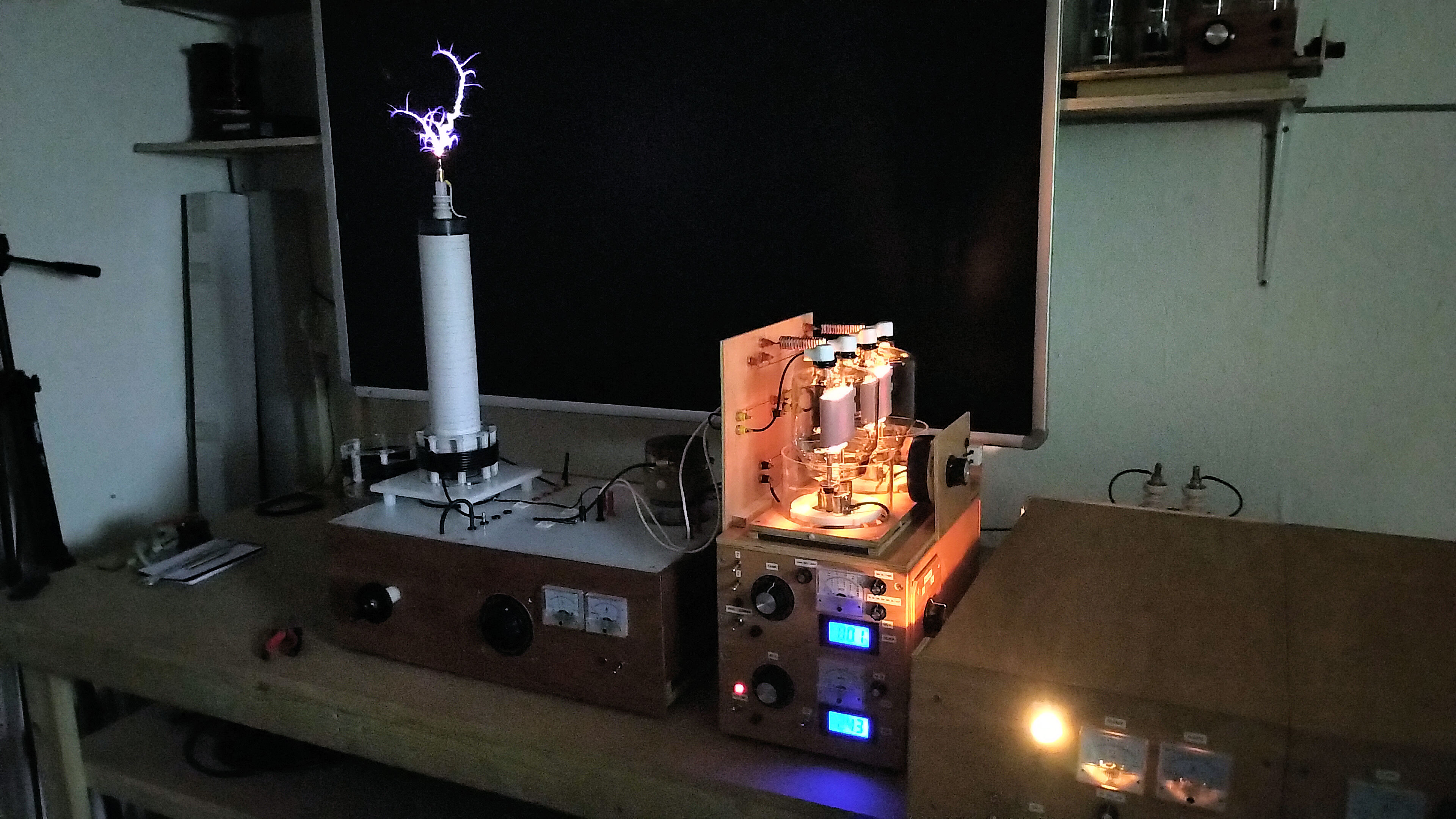
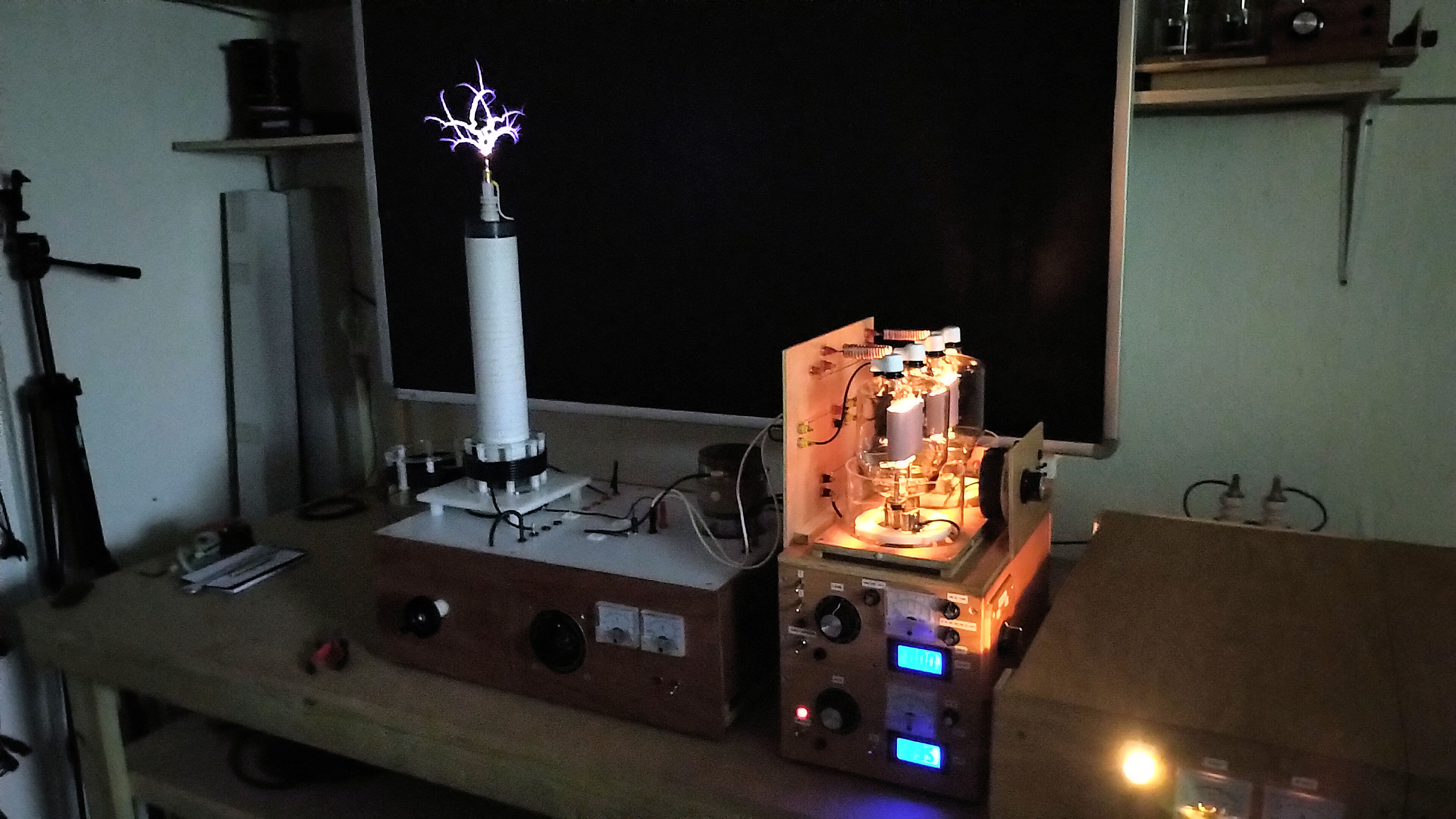
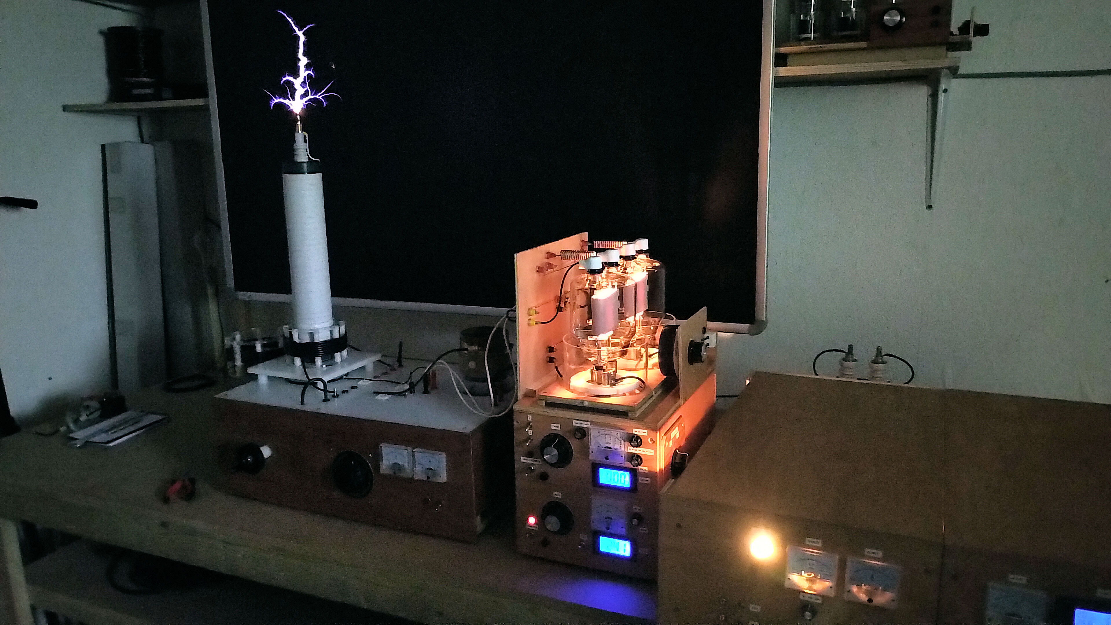
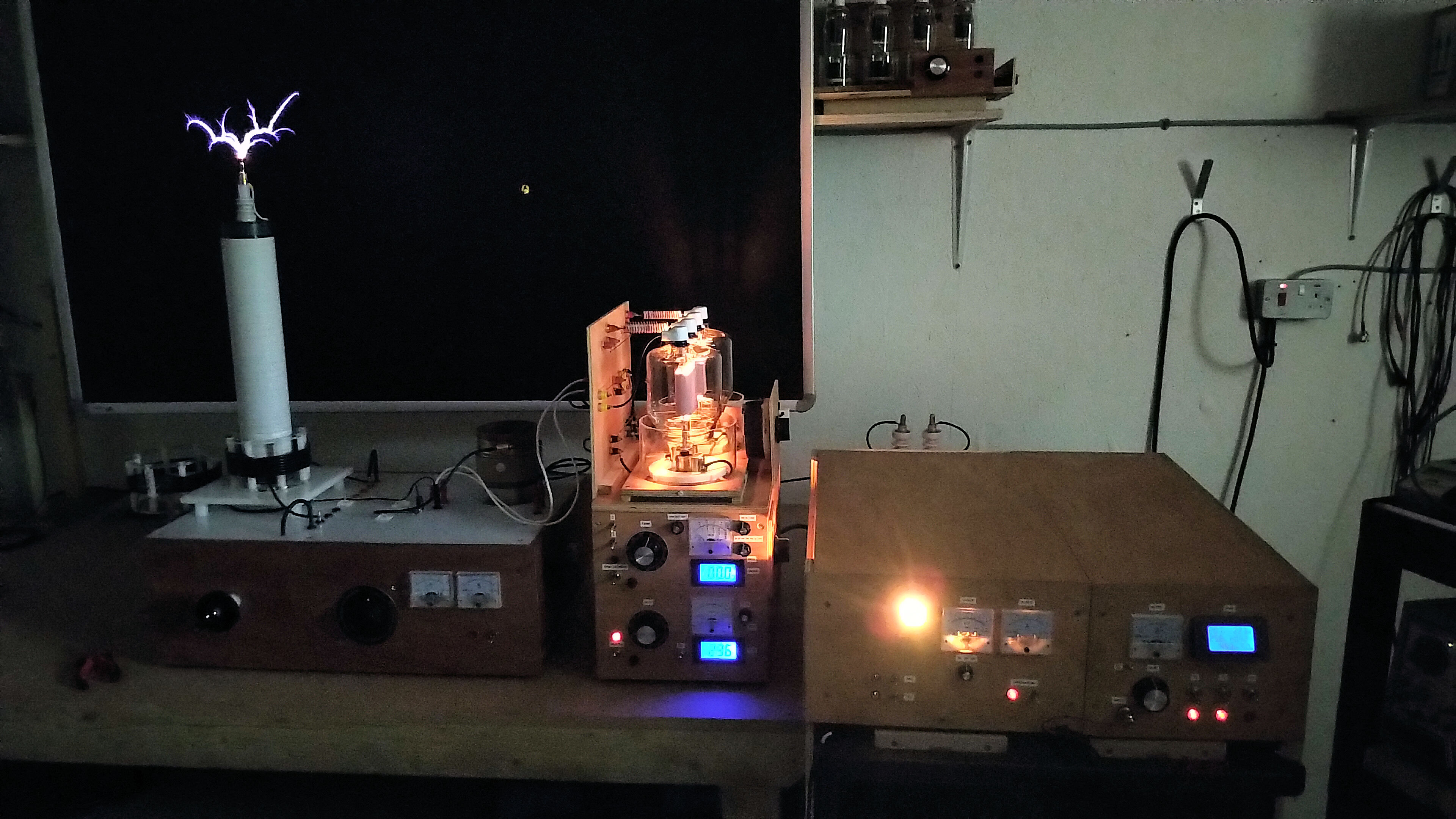
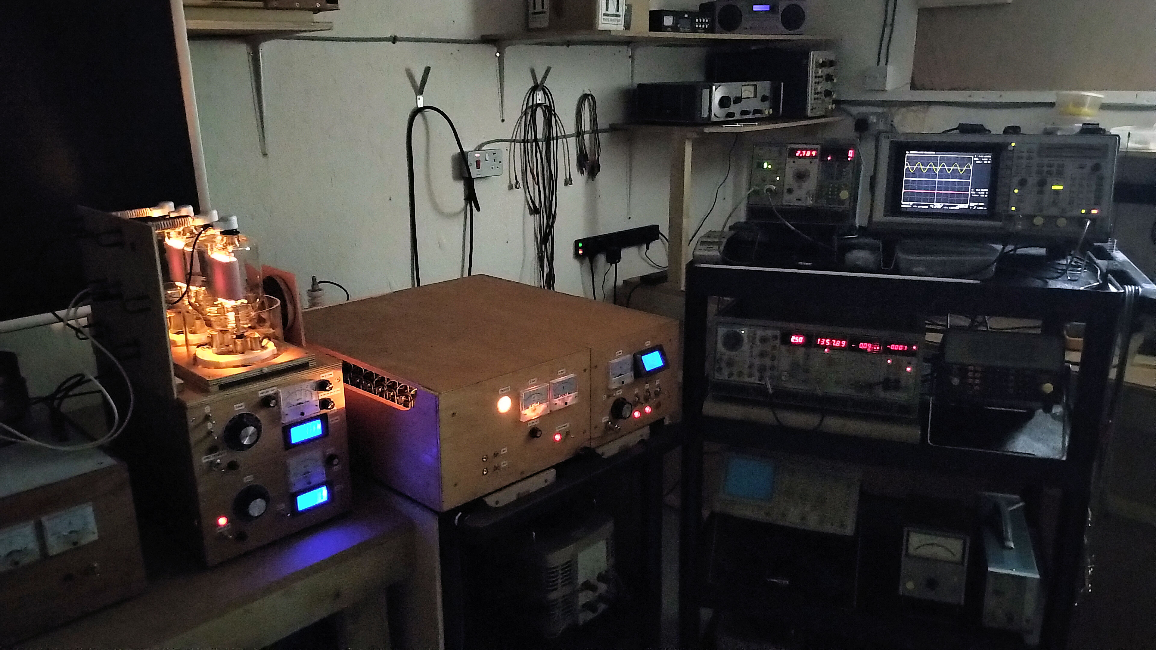
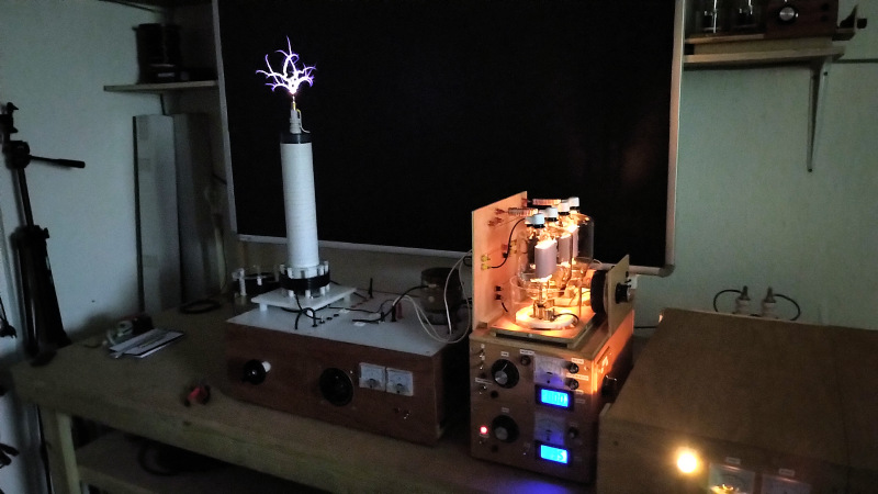
Fig. 2.1 The tube supply series setup with the high voltage & plate supply, the heater, grid & screen supply, and the dual 833C tube board. Alongside is the test equipment setup that I use to measure experiments in the displacement and transference of electric power. A motley crew of yesteryear test equipment but very accurate and reliable in the harsh environment of electricity research using Tesla coils.
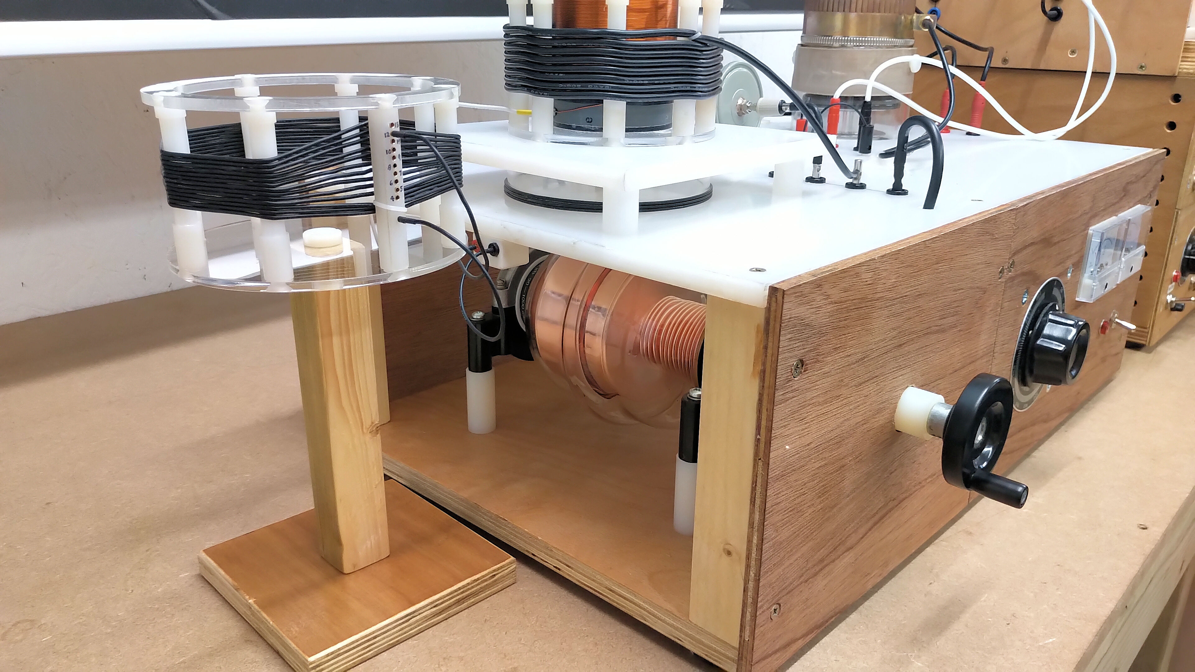
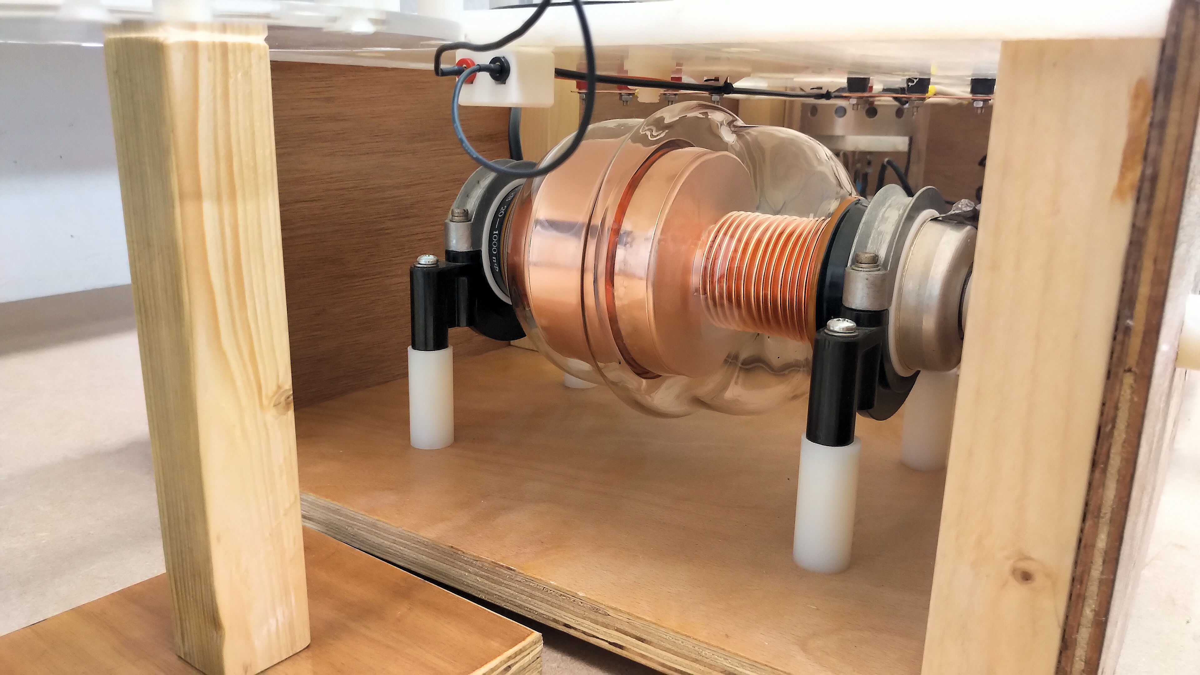
Fig. 2.2 The tube supply series setup with the Tesla coil unit used in the first of the Wheelwork of Nature series, Fractal "Fern" Discharges. Here the dual 833C tube board produces very good results with this coil unit at the upper parallel resonant frequency at ~4Mc. Using two transformers in series with the bridge rectifier the plate supply can drive the dual 833C tubes at ~4.5kV @ 2.5kW input power.
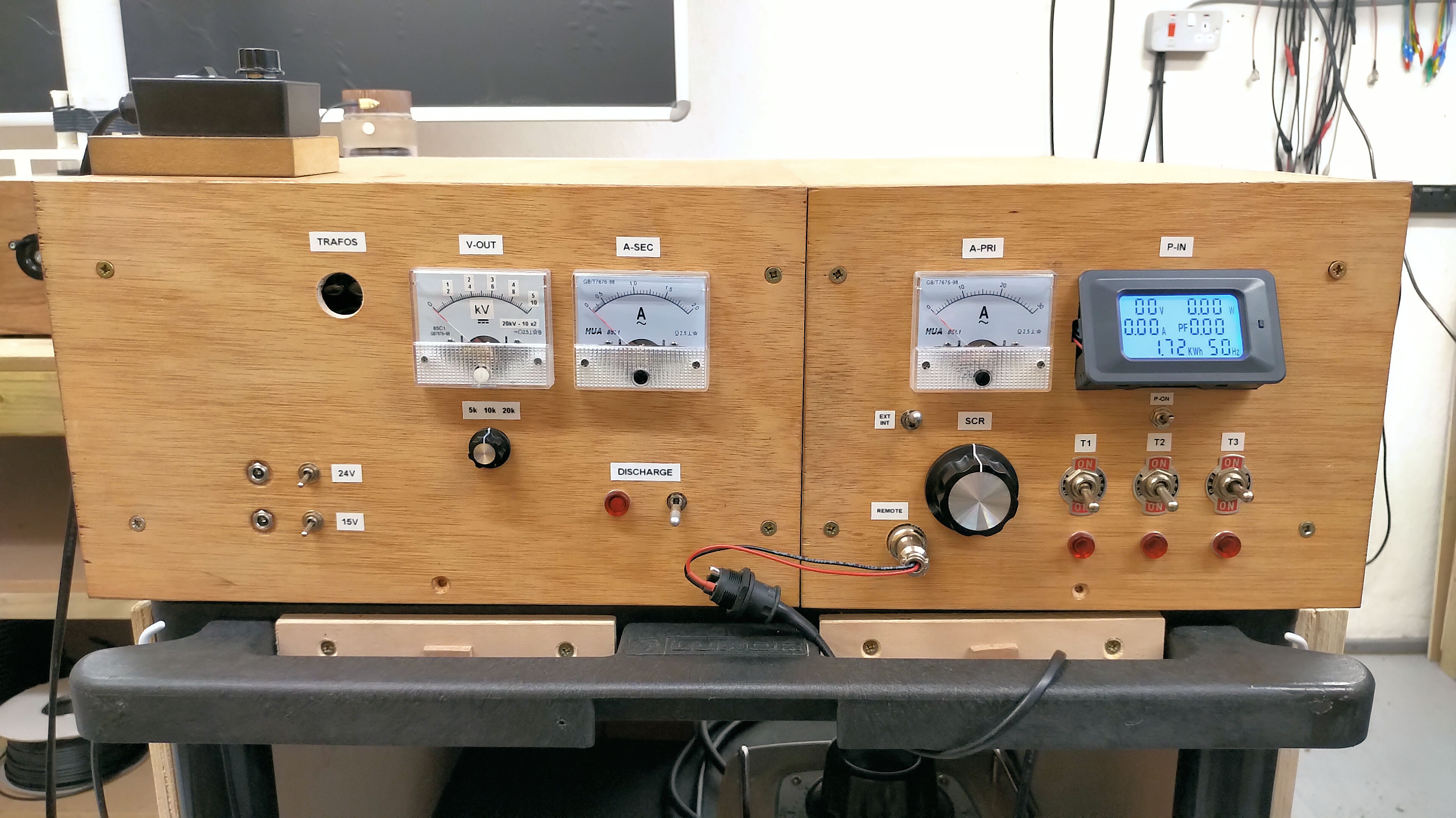
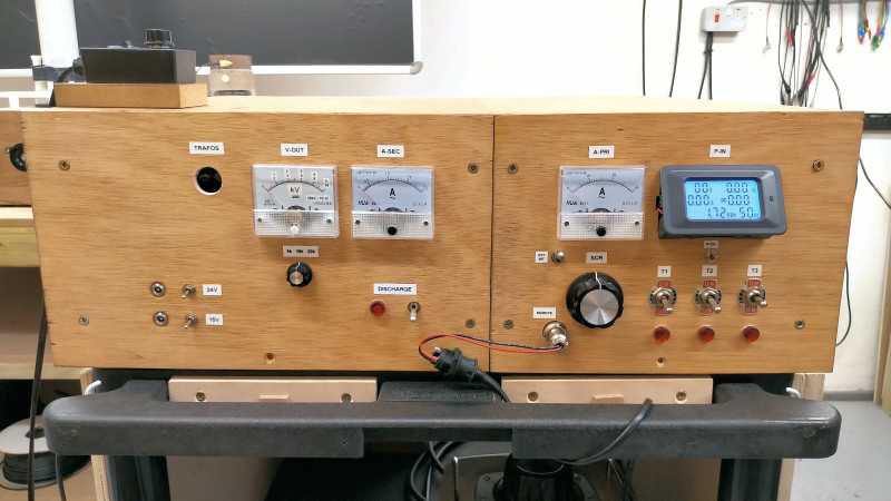
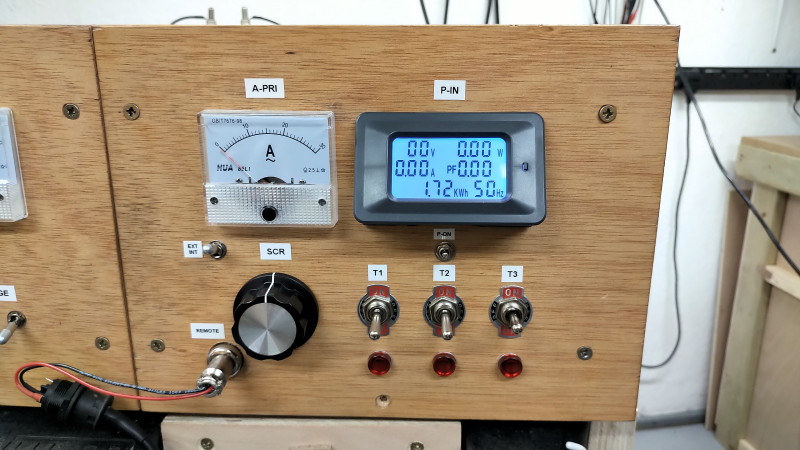
Fig. 2.3 The front panels of the plate supply showing the output monitor, discharge and low voltage outputs on the left, and the input power monitor, SCR and remote controls, and transformer phase and selection controls on the right.
Fig. 2.4 The input power control panel uses a complete digital power monitor unit which is battery powered and can continue to operate even when there is no line supply. Analogue meters are also good for safety as they require no additional power, and here monitors the total ac input current to the transformers. Transformers are selected using the three position phase/off switches.
Fig. 2.5 The inner side of the power control panel showing the battery powered power meter and current transformer, the compact and tight wiring of the transformer on-off-on switches, the SCR control wiring, and the remote control socket. The panel is designed to fold-out for easy access and maintenance, whilst still fully connected.
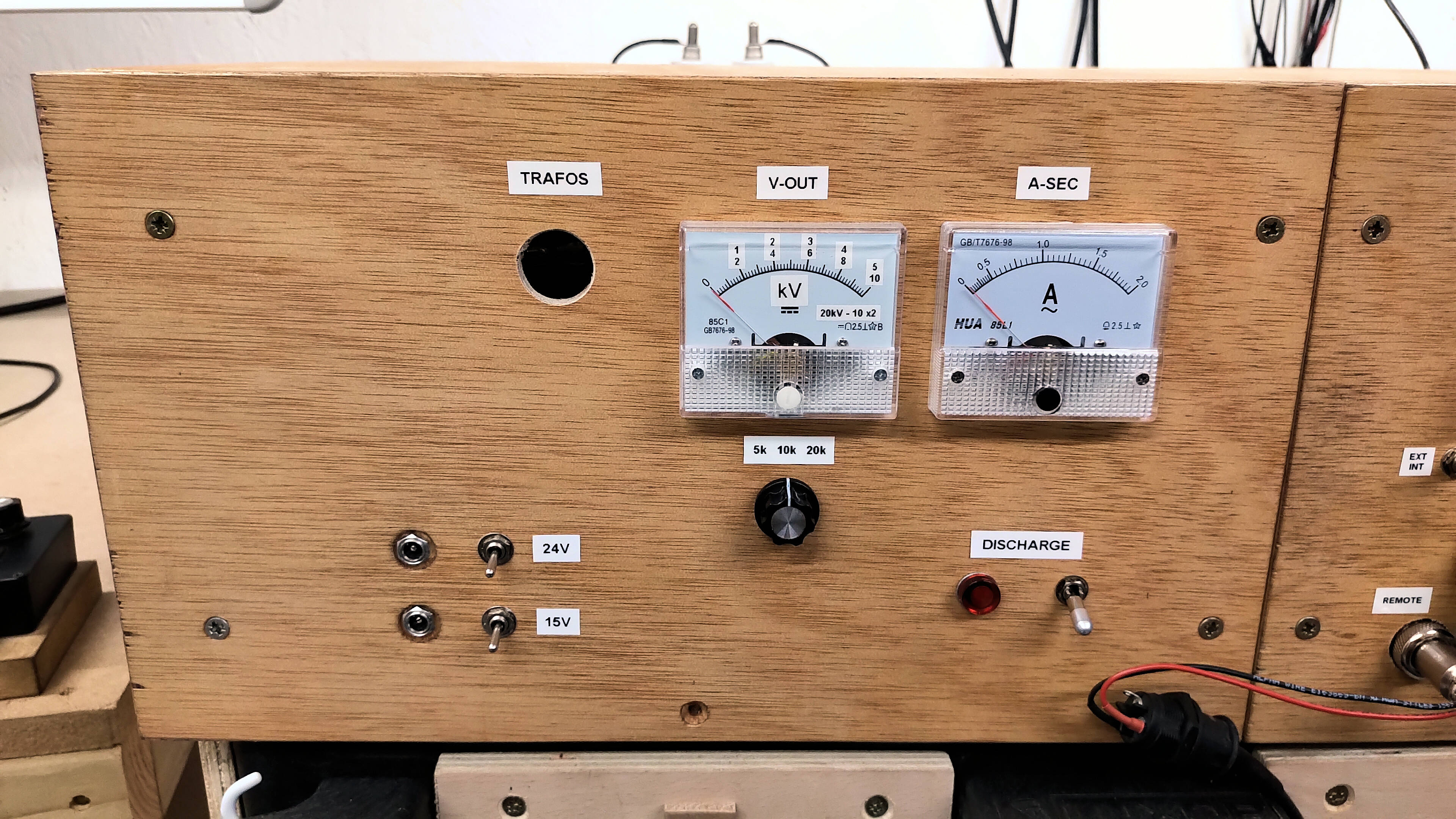
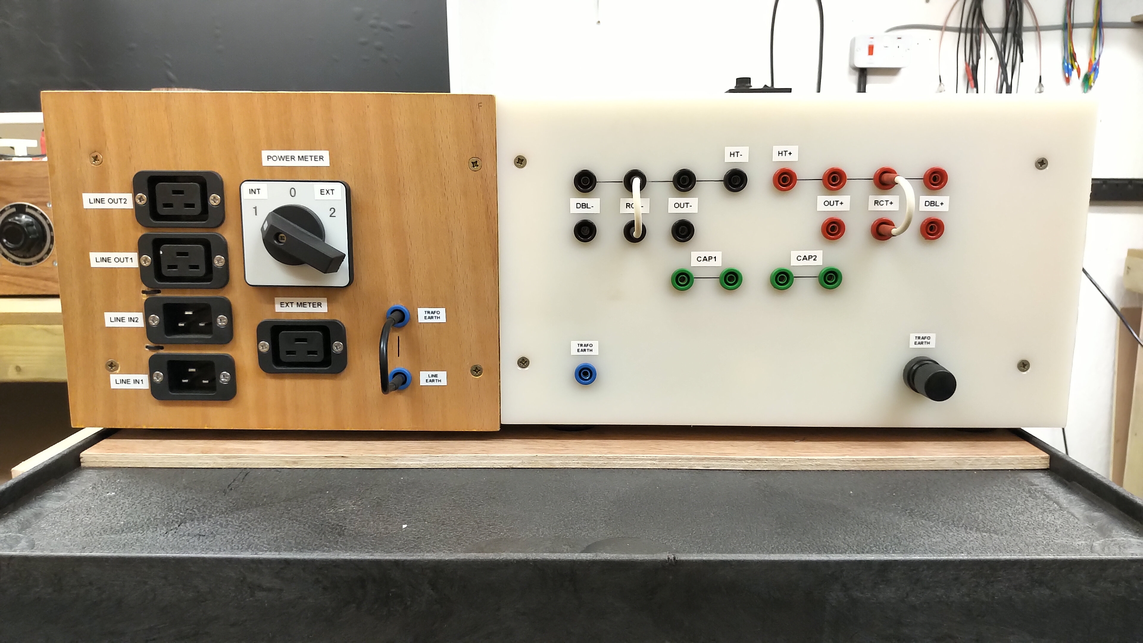
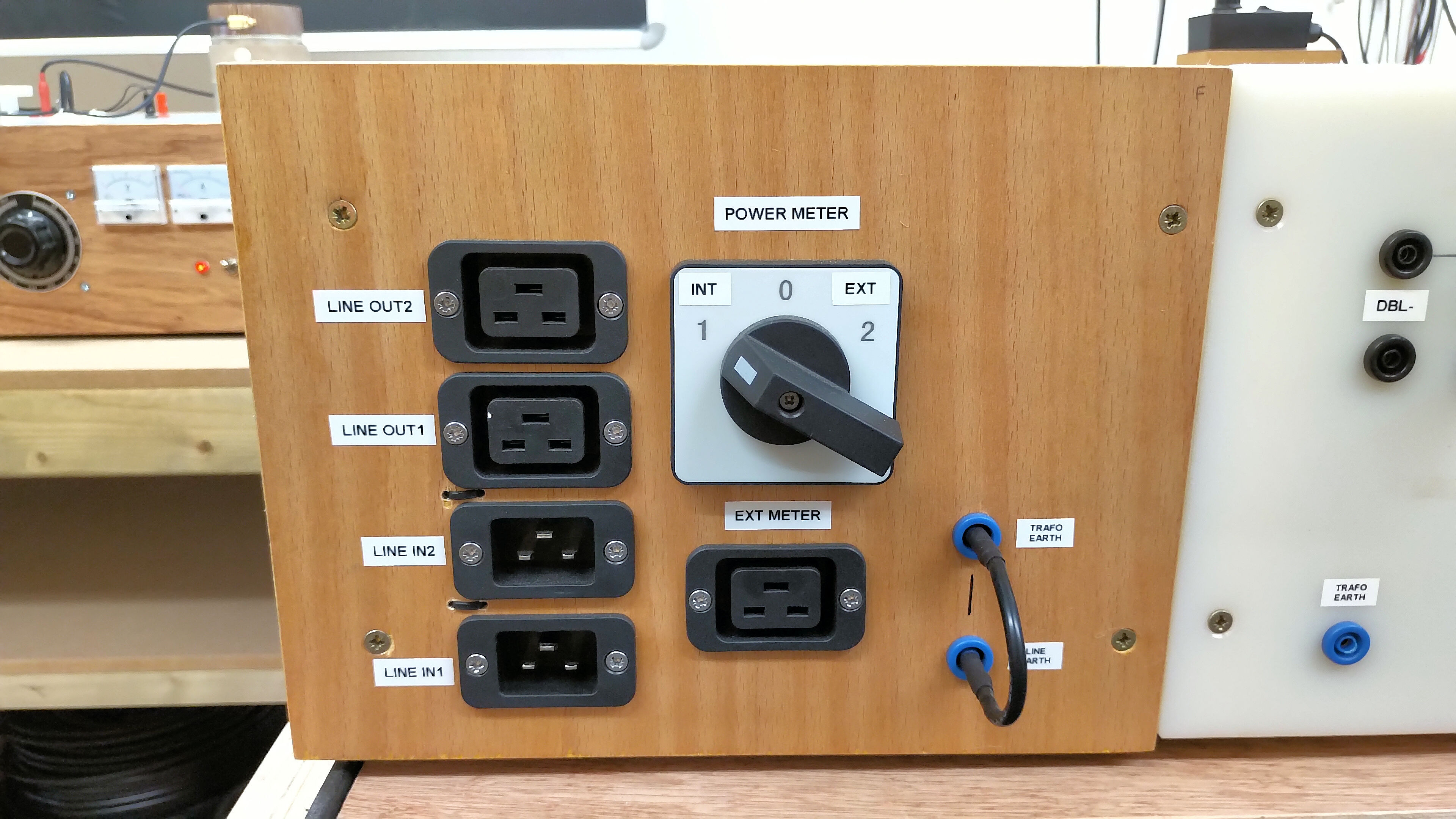
Fig. 2.6 The output monitor, discharge, and low voltage output panel. The A-SEC meter measures the secondary current at the low end of the transformer stack. The trafos light is a 230V 25W pygmy light setup to shine inside and outside as a warning that power is applied to the high voltage transformers.
Fig. 2.7 The main power panel from the outside, with primary MCB for the high voltage transformers, switch and fuse for low voltage, switched cooling fans, and final line selection that switches between the internal SCR power controller, and an external input e.g. variac. The output of the line select switch feeds the transformer control switches on the front panel.
Fig. 2.8 The main power panel folds out for easy access and maintenance. Here the internal arrangement of the components is clear, the SCR on the far right next to the MCB, and the 15V low voltage supply is positioned between the cooling fans. Forced air cooling is arranged to pass between the transformers and over the rectifier and doubler diodes.
Fig. 2.9 The rear of the pate supply showing the line supply input/output panel on the left, and the high voltage output selection panel on the right. The HV panel is made in nylon with high voltage terminals to prevent leakage and breakdown to the wooden casing at very high outputs e.g. 3-series transformers with doubler open-circuit voltage up to 18kV.
Fig. 2.10 The line supply panel uses two heavy-duty inputs with combined current handling up to 50A. Outputs are provided to chain tube series units together. A power meter selection switch is provided for internal (on the front panel), and/or external via the outlet socket. A jumper for transformer earth to line supply earth is also provided. Removing this jumper allows for floating the transformer stack.
Fig. 2.11 As with other panels, the line supply panel can be folded out whilst connected for easy access, maintenance, and measurement. The wiring is compact and neatly routed to assist in fault-finding and repair if required.
Fig. 2.12 The HT output panel uses silicone coated 20kV jumpers to patch the required internal module outputs to the final HT output. These jumpers correspond to the module input jumpers that are configured on the transformer patch board. CAP1 & 2 are for series connection of HV capacitors at the output. The HT panel is fixed and does not fold-out due to its specifically arranged and routed wiring.
Fig. 2.13 The left-hand side of the supply has the doubler unit behind it, and only acts as the vent for forced cooling air to flow out of the supply enclosure. The cooling fans are positioned on the right-hand panel on the other side and behind the HV transformers. Forced cooling passes over the transformers, rectifier and doubler diodes, doubler capacitors, and then out of the left-hand vent.
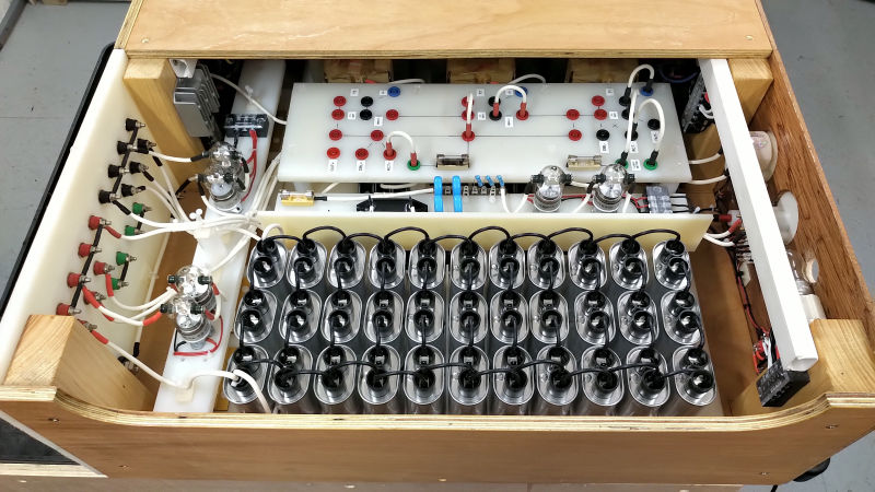
Fig. 2.14 Plate supply with the access panel removed at the top. This panel allows fast access to the transformer patch panel, the protection fuses at the transformer outputs, and the for the monitor board. This panel is sometimes removed for observation during operation when the supply is being used in adverse conditions e.g. significantly mis-matched conditions between supply, generator, and load.
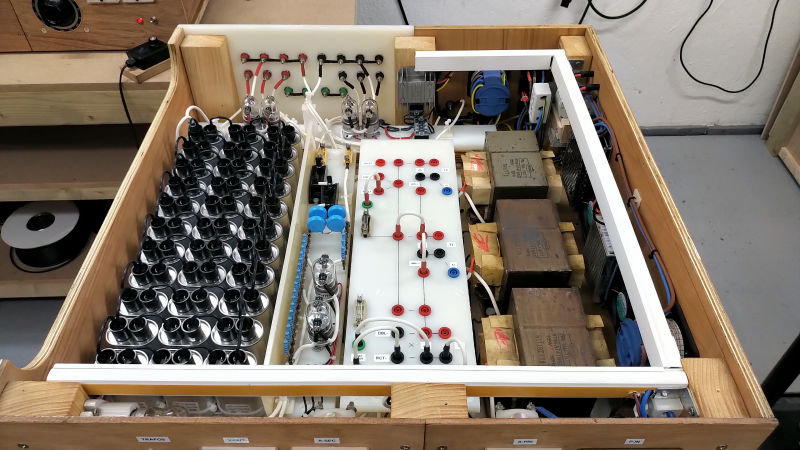
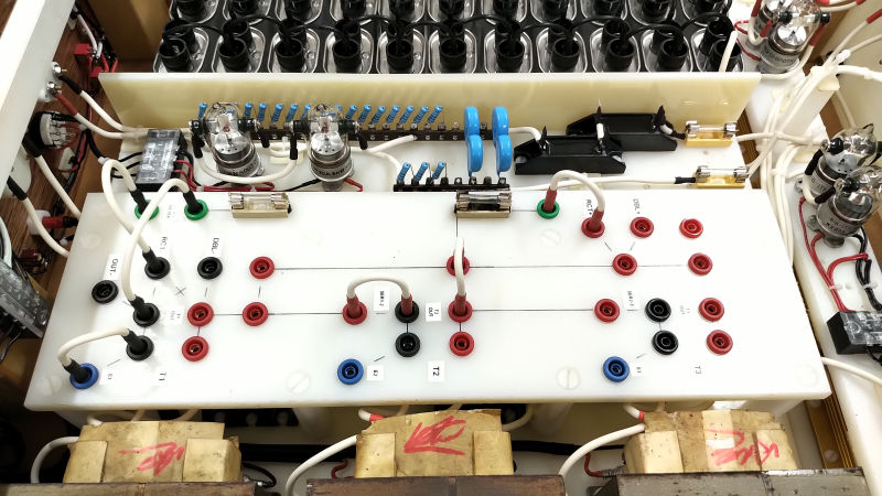
Fig. 2.15 Here the compact layout of the internal modules is very clear. The transformer patch board, monitor board, doubler board, and dischage board are all visible, and are all wired and connected using AWG16 20kV silicone coated flexible cable.
Fig. 2.16 The transformer patch board allows for a wide range of transformer parallel and series connection, fuse protection, and modular output connection. The monitor board rectifies and smoothes the HT output before reducing the current to 1mA FS for the front panel meter via a long resistor chain, switched by vacuum relays for the 5kV, 10kV, and 20kV ranges.
Fig. 2.17 Wiring around the enclosure for the line supply and low voltage is via the white conduit trunking, which safely and neatly retains wiring away from any of the HV components. Connection of the low voltage and control signals to the HV modules is via screw terminal blocks making for easy removal of any of the internal modules.
Fig. 2.18 The high voltage discharge board is included to allow for safe discharge of externally connected tank/blocking capacitors. There are many occasions in experimental research where these capacitors can be left fully charged with no easy way to discharge the enourmous energy stored. The discharge board safely switches the output to a high power resistive load via 4-series vacuum relays.
Fig. 2.19 With some of the inner modules removed the discharge board can be clearly seen, with the upper level vacuum relays, and the lower level with 5-series 100W power resistors with high voltage withstand. This discharge unit can be used safely up to 15kV, and is powered by the 24V dc-dc converter (ribbed silver module) that is mounted on the support pillar centre-right of the picture.
Fig. 2.20 An overall internal view of the plate supply with all top panels removed. The logical arrangement of the inner modules combined with easy side panel access, make this powerful yet compact design easy to access and maintain, and trouble shoot operation and performance problems if and when they arise.
Fig. 2.21 A clear view of the monitor board between the transformer board and the doubler board. The halfwave rectification and smoothing allows for a maximum DC level indication of the peak HT envelope on the front panel. This is effective even when the output is a sinusoid or complex chopped waveform when using the SCR power control.
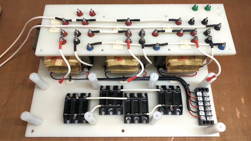
Fig. 2.22 The transformer board removed from the supply, and with the patch board folded back onto the transformers, showing how the patch board is wired, the high voltage bridge rectifier, and the line supply inputs for the transformer primary coils.
Figures 3 below show the complete circuit diagrams for the high voltage and plate supply across three sheets. The high-resolution versions can be viewed by clicking on the following links Fig 3.1, Fig 3.2, and Fig 3.3.
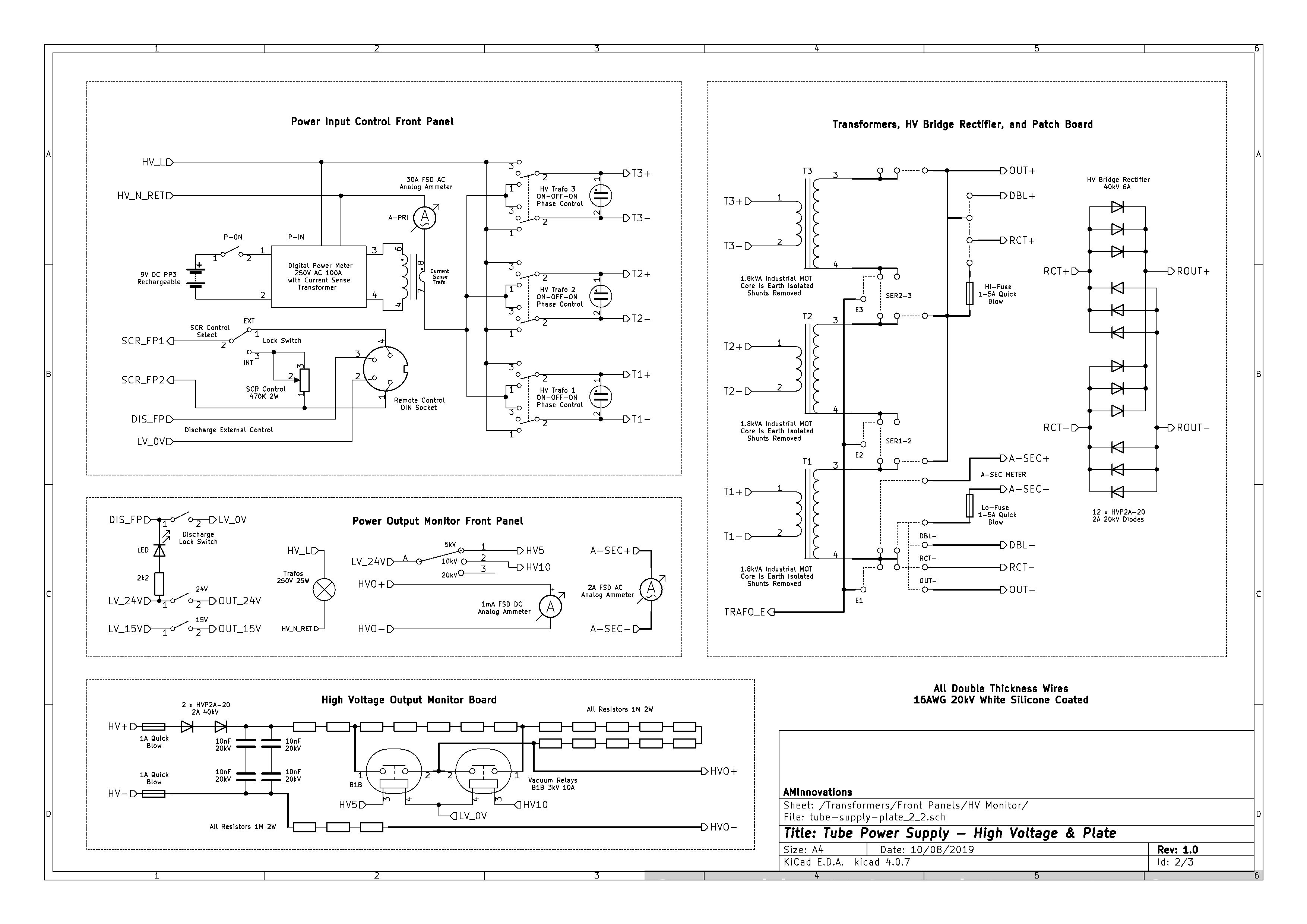
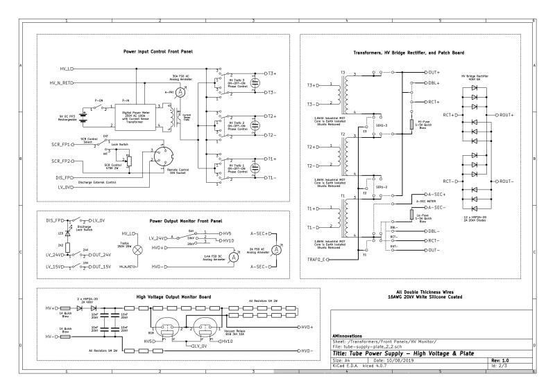
Fig. 3.1 Tube High Voltage & Plate Supply schematic showing the Power Input Control Front Panel, the Transformers, HV Bridge Rectifier, and Patch Board, the Power Output Monitor Front Panel, and the HV Output Monitor Board.
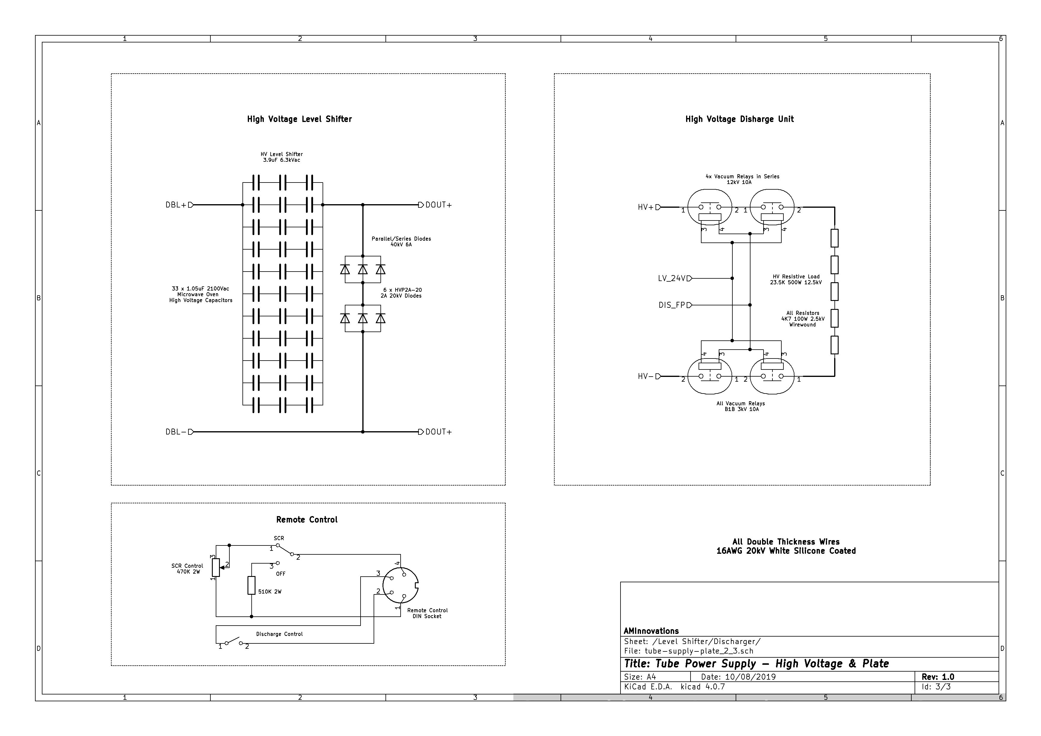
Fig. 3.2 Tube High Voltage & Plate Supply schematic showing the HV Level Shifter, the HV Discharge Unit, and the Remote Control.
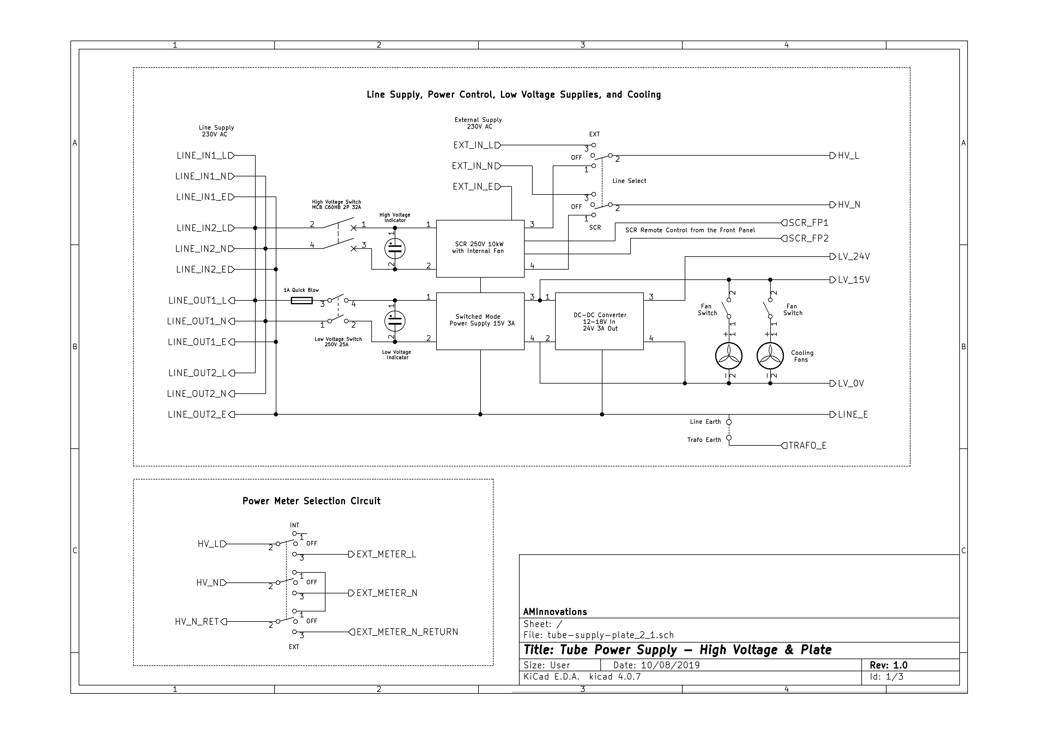
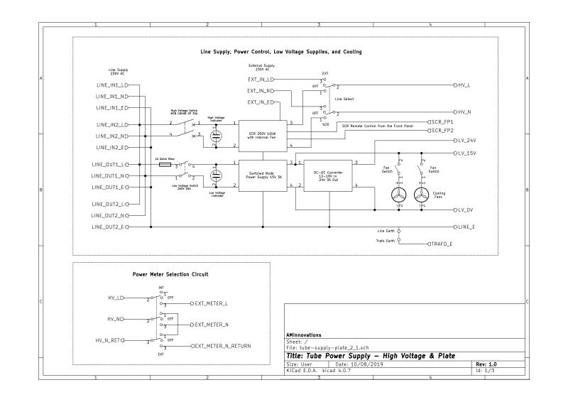
Fig. 3.3 Tube High Voltage & Plate Supply schematic showing the Line Supply, Power Control, Low Voltage Supplies, and Cooling, and the Power Meter Selection Circuit.
Principle of Operation – General Summary
In principle the plate supply is very simple consisting of three microwave oven transformers that can be easily connected in a variety of parallel and serial configurations. Power is provided to the transformers from the line supply and via a high power SCR control unit equivalent to a powerful light dimmer control, or from an external source such as a variac or other type of power controller. The selected line supply is then fed to the three transformer power switches on the front panel. These three position switches have a centre off position, and then on position either both up and down. The on positions are arranged to swap the live and neutral connections to the transformer so changing the phase of the line supply to each transformer. The change in phase of the line supply allows transformers to be configured in different arrangements both as positive and negative output with a centre ground point. This is particularly useful in the case of the three series transformers where maximum voltage from core to primary needs to be restricted. This is covered in detail in a later section below.
Phase controlled line supply is then fed from the front panel to the transformer board primary coil circuits. The patch board allows for configuration of the connections on the secondary coil side of the transformers. The output of the patch board feeds various different modules including direct output, the HV bridge rectifier, and the HV level shifter. The selected module is finally connected to the final high tension (HT) output via a second patch board on the HT rear output panel. The HT output is then also connected to the HV discharge board, and also to the HV output monitor board. The HT output board also provides intermediary connections for tank/blocking capacitors facilitating the series and parallel connection of large HV capacitors safely and in close proximity to the power supply outputs. The wooden enclosure is so arranged to accommodate other devices in the tube power supply series, as well as open access to the main components through a large access panel in the top of the plate supply. In extreme operating and prototype conditions I often run with this access panel open (and via remote control) in order to watch for any unusual or unexpected effects.
The complete supply is housed in a varnished wooden casing, and internally arranged and assembled to be easy to repair, maintain, and modify. Module boards can be easily removed internally, and side panels fold open whilst still electrically connected for easy measurement and fault diagnosis. It should be noted that this type of power supply is designed for research prototyping and hence encounters a very wide range of different loading and matching, all the way from an open circuit condition on the output, through to heavily overloaded current conditions, and very high reflected RF and transient power conditions. These extreme operating conditions necessitate that the power supply is easy to diagnose, adjust, and repair internally, and hence it is arranged and assembled accordingly with easy access to all critical internal systems.
Power Input and Control Panel
Fig 3.2 shows the circuit diagram for the Line Supply, Power Control, Low Voltage Supplies, and Cooling. The line supply from the rear input panel provides both line supply outputs for chained connection of other modules, devices, and instruments, and internally splits into two feeds, one for the HV supply, and one of the low voltage (LV) supply. The LV supply is fused and switched with a LV indicator to show active operation. The LV line supply feeds a 15V 3A switched mode power supply which powers all the internal LV components, and also has external outputs to power other LV devices and modules in the experimental setup. Internally the 15V is stepped up to 24V by a DC-DC converter. The 24V is suitable to switch the W1W or B1B vacuum relays which operate quickly and reliably at the higher voltage. The internal cooling fans are both switched and are powered from the 15V LV supply. The fans are especially necessary during prolonged high power usage, and are positioned directly behind the HV transformers.
The HV supply is protected by a dual-pole 32A MCB, (upgradeable to 40A MCB in extreme conditions), and with a neon indicator to show active operation. The HV line supply is fed directly to a 250V 10kW SCR which is arranged for both internal and remote control via the front panel. The SCR provides progressive power control for HV transformers which is often most necessary for microwave oven transformers that have had their magnetic restriction shunts removed. The SCR voltage profile is also highly non-linear which in some experiments like Tesla’s Radiant Energy and Matter, and Displacement and Transference of Electric Power series, is most useful to reveal, accentuate, and maximise certain types of phenomena including displacement and radiant energy, and dielectric induction field charging and storage. The SCR output is fed to a line supply selection which switches either the SCR output or external line supply input to the power control front panel. The line supply selection was included to allow for quick switching to a variac for progressive linear control of a sinusoidal line supply which is most useful during experiments with phenomena that vary with supply voltage profile.
Fig 3.1 shows the circuit diagram for the Power Input Control Front Panel which consists of the following:
1. The three off and phase control transformer switches. Line supply from the selection switch on the main power panel is fed to the switches each with three positions, off and up and down, where the up and down positions switch the line supply to the respective transformer, and also swap the live and neutral from up to down to control phase control of the transformer primary. Each switch is accompanied by a neon indicator that both shows if the transformer is currently active, and the intensity that the transformer is being driven.
2. The digital power monitor is 9V battery driven in order to have independent operation from the line supply, and continues to be active even if the line supply is removed, this is important for safety in the event of a fault where the line supply is still connected to the rear panel, but has become disconnected internally due to say an SCR open circuit fault, and line supply to the transformers can still be monitored. The digital power monitor takes input directly from the line supply fed to the front panel for voltage, and for current via a current transformer in the neutral line supply return, and mounted to the inside of the power control panel. The meter has an on-off switch P-On, and is also angled upwards in the panel for easy reading. The meter provides a useful real-time summary of all operating measurements on the line supply side, including apparent voltage and current, real power indication and consumption, and total power factor.
3. The neutral line supply return also includes a 30A AC meter which is particularly good for quick monitoring of the total transformer primary current. This is useful in high current drive scenarios when changes in tuning can easily place the power supply in a very different operating condition, where very large currents are suddenly drawn from the line supply e.g. whilst tuning through the transition between the lower and upper parallel resonant modes of a Tesla coil whilst driving at moderate to high-powers > 1kW.
4. A locking switch to change from the internal SCR control potentiometer to the external remote control potentiometer. The switch is locking in order to avoid accidental switching which could yield dangerous and unexpected results if the SCR suddenly was switched to a higher power condition. The selected potentiometer connects directly back to the SCR on the main power panel and controls progressively the active portion of the line supply cycle that is fed to the transformers.
5. The remote control socket is a 10-pin connector which currently has 2 lines for the SCR remote potentiometer, and 2 lines to switch the HV discharge module on and off. The other 6 lines are not used and available for future expansion and functionality.
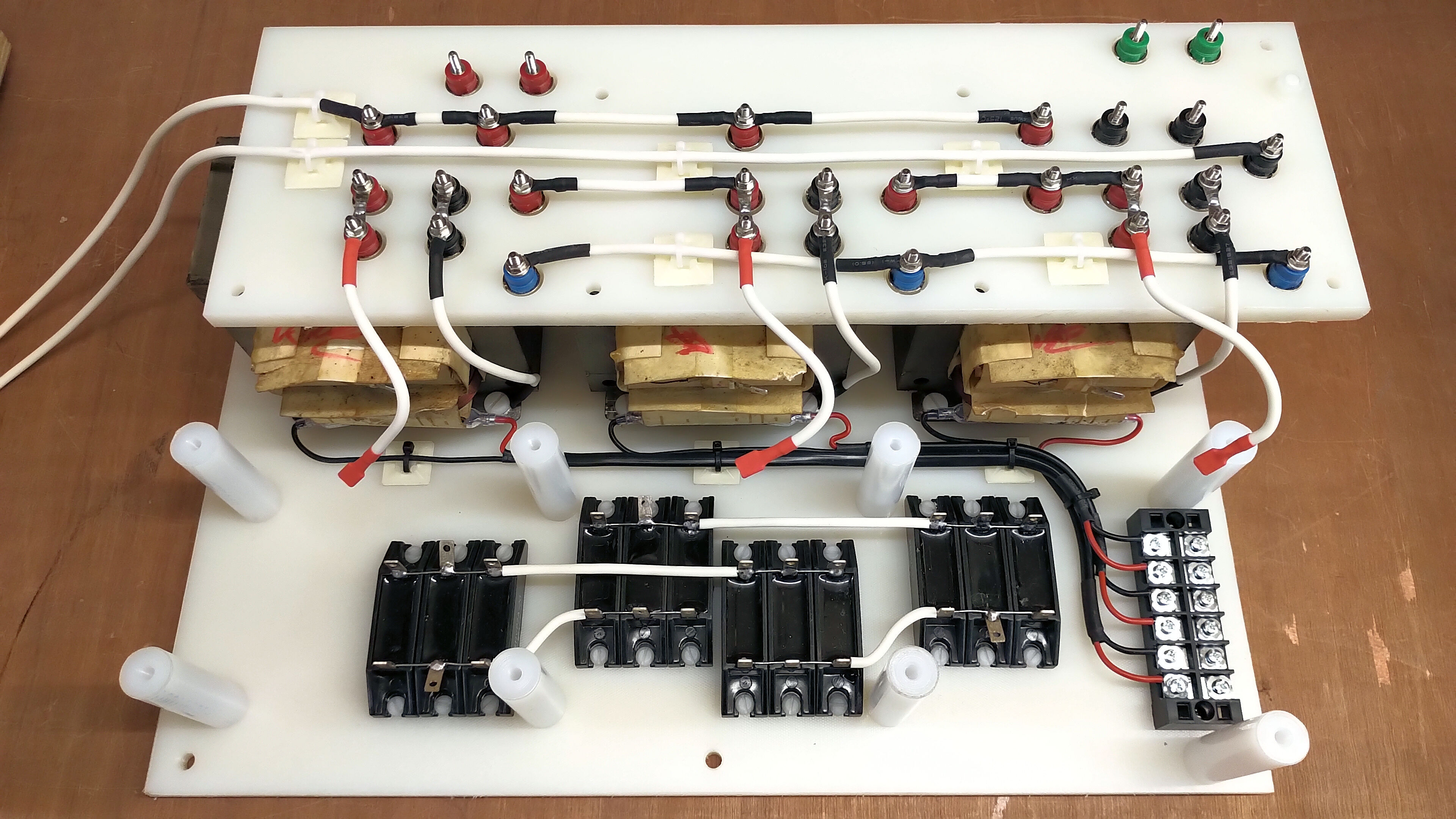
Transformers and Patch Board
Fig 3.1 shows the circuit diagram for the Transformers and Patch Board. The microwave oven transformers (MOT) are a heavy-duty industrial type rated to 1.8kVA with the magnetic shunts removed. A traditional MOT is a cheap high voltage transformer manufactured with the minimum weight of copper and hence cost, and designed to match the very specific impedance of a magnetron when correctly matched using the level shift capacitor. The cheap construction of the transformer usually involves welding the laminated metal core together on both sides, which whilst simple to make, results in shorting out much of the laminated core reducing it electrically to a large block of magnetic material that will easily saturate when sufficient power is applied to the primary coil. In this basic form the MOT does not easily lend itself to a progressive linear power supply at high voltage, like other types of high voltage transformers. The MOT however does benefit from being very robust and also able to supply high currents up to easily 1A at around 2kV AC.
The magnetic shunts are so arranged during manufacture of the MOT to reduce the free magnetic coupling between the primary and secondary coils, and hence limit the power transfer from primary to secondary, driving the magnetron impedance efficiently, without core saturation and hence excessive heat generation, and without pulling excessive current from the line supply. When reused as a high voltage transformer in this type of plate supply the magnetic shunts restrict significantly the maximum power output performance of the transformer, and need to be removed carefully (to avoid damaging the windings), with a drift and heavy mallet. I made up a wooden jig screwed to the bench to hold the transformers securely whilst driving out the magnetic shunts. The un-shunted MOT now benefits from no restrictive magnetic coupling, but does now need to be current limited to prevent excessive core-saturation at the top-end of the line supply input, and with higher impedance loads at the output of the generator e.g. a vacuum tube generator.
Current limiting can be achieved a variety of ways, including chokes in the primary and/or secondary coil circuits, but in this plate supply I use an SCR power controller which provides progressive power output by varying the active line supply cycle. The SCR introduces large non-linear distortion in the line supply to the transformers which is both a hindrance in some experiments and requires to be smoothed with large HV capacitors, or a benefit in generators designed to emphasis certain non-linear phenomena e.g. displacement and radiant energy experiments. Oscilloscope waveforms of the SCR drive of a MOT, and for more details on using a MOT as a high voltage transformer see High Voltage Supply. Overall the MOT when correctly used and setup is a very robust and high power transformer, which with cooling can run at very high output powers for sustainably long time periods. Combinations of MOTs in parallel and series can generate a wide range of high current and high voltage outputs, which is the principle I have used in this high voltage plate supply.
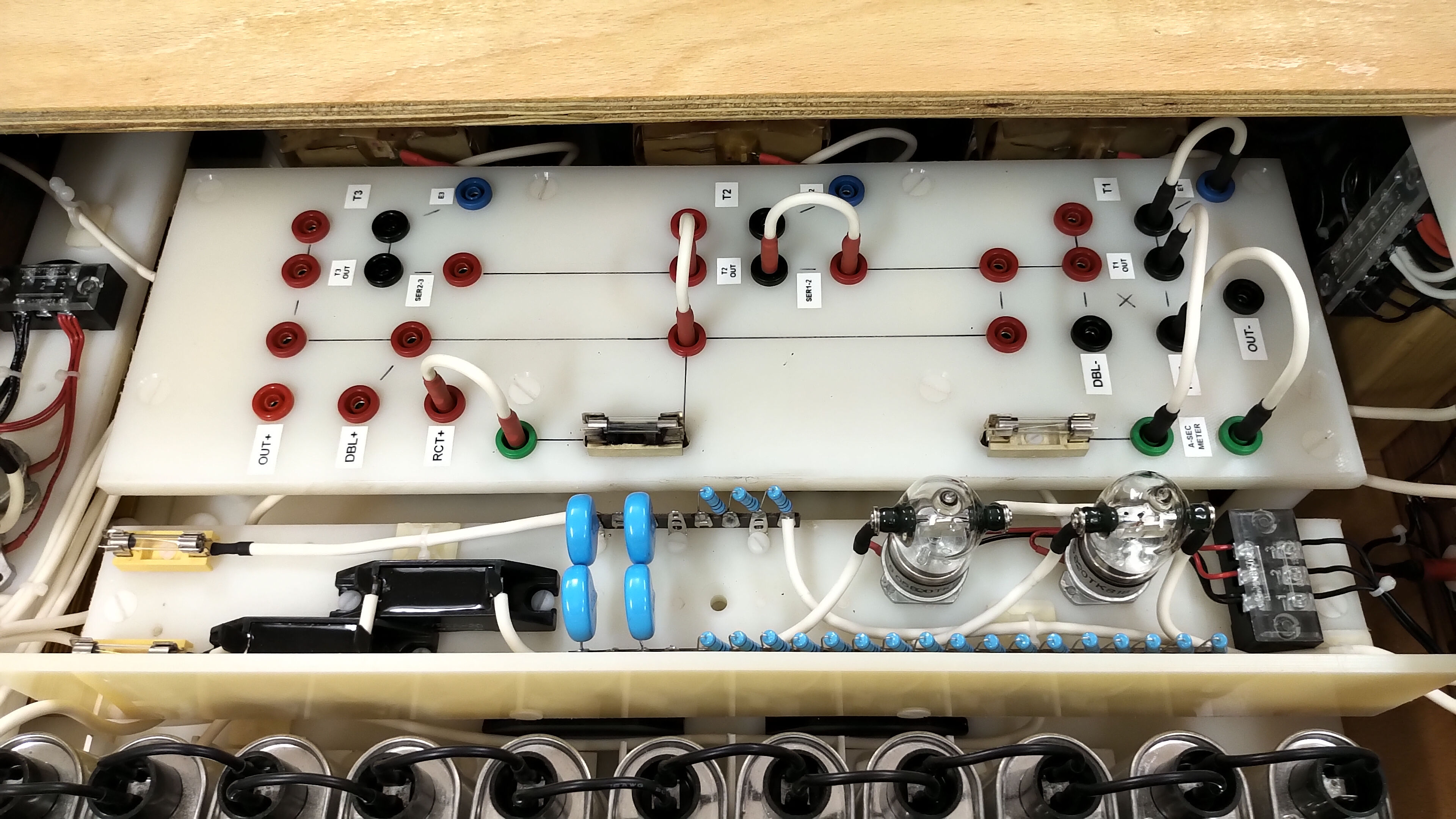
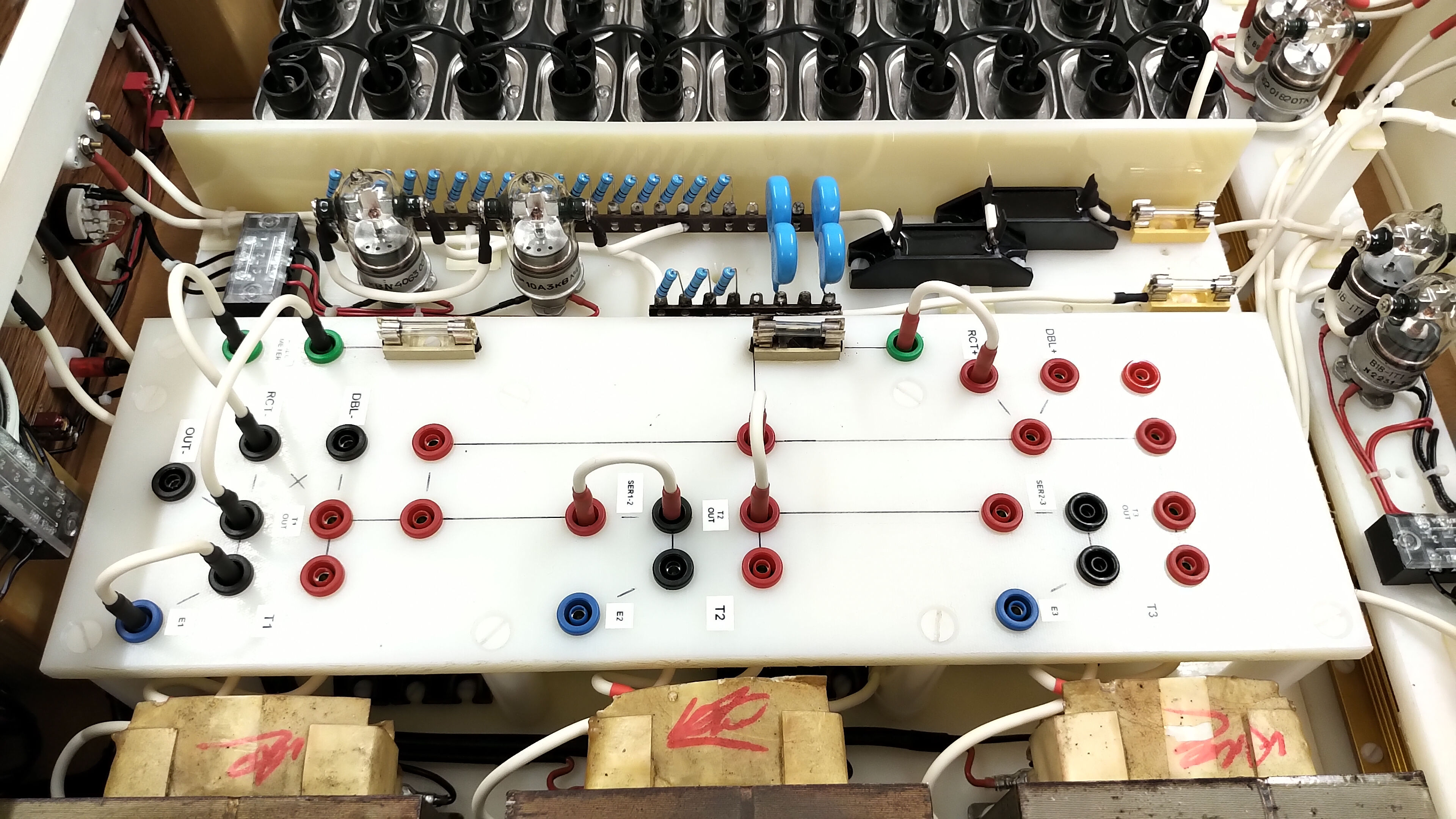
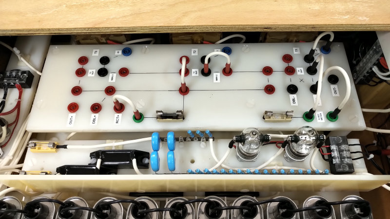
The three MOTs are switched independently from off to specific line supply phase (live and neutral connection to the primary) by the three toggle switches T1 to T3 on the power control front panel. The MOTs themselves are physically arranged on a nylon plastic sheet so that the MOTs cores are not electrically connected. The core of a MOT usually forms one terminal of the high voltage output, the inner end of the secondary being connected directly to the core. In this way the transformers can be isolated from each other and then connected via the patch board into different combinations of single, parallel, or series connected. Configurations of the transformers using the patch board is detailed in Figures 4, and further discussed below in that section. The patch board provides both connection of the transformers together in different configurations, and also connection of the the configured transformer set to the various internal modules of the power supply as follows:
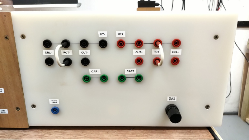
1. The OUT+ and OUT- terminals take the raw transformer output directly to the HT output board, and allow for direct drive at the output from the transformers.
2. The RCT+ and RCT- terminals connect the transformers to the HV bridge rectifier inputs, and its outputs are connected to the HT output board.
3. The DBL+ and DBL- terminals connect the transformers to the HV level shifter inputs, and its outputs are connected to the HT output board.
There are two protection fuses at the high-side and low-side of the transformer outputs and prior to connecting to any of the internal modules or HT output board. The high-side fuse is particularly good to prevent excessive current draw through the bridge rectifier and level shifter diodes, whereas the low-side fuse is particularly good to prevent spike surges from the transformers and through the diodes, when for example a vacuum tube oscillator stops oscillating at high output power, and then suddenly restarts oscillating. Both high-side and low-side fuses are necessary to protect the supply from a range of different operating fault conditions, which is very important in extreme research and prototype operating conditions. I lost one set of bridge rectifier diodes (12 x HV diodes) before I used the high and low side protection fuses. A 2A FSD AC analogue meter is connected in series with the low-side fuse, which gives an average approximation of the secondary current being drawn from the complete transformer setup. The inter-connection of the patch board, outputs, and meter is via 4mm plugs with 20kV 16AWG wire.
High Voltage Bridge Rectifier
Fig 3.1 shows the circuit diagram for the HV Bridge Rectifier, which is mounted below the patch board on the transformer module, and shown in detail in Fig 2.22. The rectifier is nominally 40kV @ 6A and is constructed from 12 x HVP2A-20 20kV 2A diodes. The diodes are mounted directly down to the nylon transformer board and again connected to the patch board and HT output board using 20kV 16AWG wire. Whilst quite well rated for the overall performance of the plate supply, semiconductor diodes are sensitive devices and easily blown short-circuit by over-current conditions, and blown open-circuit by HV spikes, transients, and non-linear power reflections from the experiments.
To protect these diodes, we use both the high-side and low-side fuses on the patch board, and also most importantly a blocking/tank capacitor at the HT output board. This capacitor significantly helps to prevent reflected transients and non-linear voltage spikes from the experiment and generator from passing back into the power supply and causing problems for the sensitive semiconductors. Typically for many experiments using a vacuum tube generator, and when a smoothed DC plate supply is not required, I use a 25kV 25nF pulse capacitor as the block capacitor at the HT output board. For DC smoothed plate supply I tend to use two 4kV 60uF capacitors in series to create a 8kV 30uF tank reservoir. A large tank like this needs very careful connection and discharging, which is one of the primary reasons a discharge unit is included in the power supply.
Overall when used with the blocking capacitor the HV bridge rectifier is robust and reliable, and can provide sustained high output power with only moderate heating of the diodes. These rectifier diodes are also in direct line of the forced cooling between the MOTs which makes for a high power high voltage rectified and smoothed DC plate supply or HV source. I have only lost one set of diodes before I had the high and low-side protection fuses installed, when operating at almost full power input and the vacuum tubes stopped oscillating during a tuning experiment. When it started oscillating again the current surge from the transformers at an almost full input power of 5kVA blew all 12 diodes short circuit. The high and low-side fuses now provide adequate protection against this fault condition, and I usually run with protection fuse ratings between 1-3A dependent on the transformer configuration, required output power, and type of generator e.g. vacuum tube, spark gap, impulse etc.
High Voltage Level Shifter (Doubler) Board
Fig 3.3 shows the circuit diagram for the HV Level Shifter or Doubler. The large microwave oven capacitor bank and 6 HV diodes that constitute the level shifter are mounted on its own nylon board, and are shown in detail in Fig 2.15. The principle of the level shifter is that in one half cycle of the secondary output the capacitor bank is charged up to the peak potential of the half-cycle e.g. 2.1kVRMS for a single transformer, and in the second half cycle a diode is used to raise (or lower dependent on the direction of the diode) the potential on the output of the capacitor bank by the maximum potential of the second half-cycle e.g. a further 2.1kVRMS for a single transformer. The overall result for a sinusoidal primary coil line supply input is an secondary output sinusoidal that is level shifted either up or down by the maximum potential of one half cycle of the waveform.
With a positive orientated diode direction this will produce a sinusoidal from 0V to 4.2kVRMS or ~6kV peak voltage when unloaded. In other words the secondary coil output waveform is level shifted either positive or negative dependent on the diode orientation, and hence why this circuit setup is properly known as a level shifter. This circuit is often referred to as a voltage doubler, but diverges slightly from a true doubler that uses multiple diodes and produces a rectified and doubled, or tripled etc. output dependent on the number of capacitor diode stages in the voltage multiplier. In this power supply I use the diode in the positive orientation to produce a positive level shifted output which can be selected using DBL+ and DBL- on the transformer and HT output boards. It is not without a sense of irony that I refer to the terminals as “DBL” or short for doubler!
The capacitor bank is an MMC type arrangement that consists of many microwave oven capacitors combined together to produce a higher capacity capacitor, and at a higher voltage. In this case I am using a bank of 3 x 1.05uF 2.1kVRMS capacitors in series to give a 0.35uF 6.3kVRMS single bank. With 11 of these banks combined in parallel the final capacitor bank is ~ 3.8uF @ 6.3kVRMS. When used in a level shifter configuration as shown in the circuit diagram this capacitor bank with 3 series input transformers can give a measured total level shifted output potential of up to 13kV @ 300mA, 15kV @ 150mA or almost 18kV peak open circuit potential. The diodes are again the same as those used in HV bridge rectifier and are arranged in 2 series banks of 3 in parallel to provide a 40kV 6A level shift diode.
High Voltage Monitor Board and Panel
Fig 3.1 shows the circuit diagram for the HV Output Monitor Board (HVOM), which is designed to safely provide a measure of the HT Output on the Power Output Monitor Front Panel, also shown in the circuit diagram. The HVOM circuit uses a HV half-wave rectifier using 2 x HVP2A-20 in series making a 40kV 2A rectifier diode. The rectified waveform is smoothed by an HV capacitor bank of 2 series and 2 parallel capacitors to form a 10nF 40kV smoothing capacitor bank. The rectifier and smoothing capacitor together turn the output waveform into a peak DC level which will be displayed on the front panel V-OUT meter as shown in Fig 2.6. The high voltage peak DC level is converted to a low current by a long series resistor chain, where each resistor is 1MΩ 2W. 20 series resistors together form the highest 20kV range and reduce the current from the rectifier to 1mA for 20kV. This dramatic reduction in current reduces the ripple on the peak DC to a very low level, and also safely converts the HT to a low current that can be passed to a meter on the front panel.
The meter on the front panel is a 1mA FSD DC analogue meter with its range updated to show kV rather than mA. So on the highest range 20kV at the HT Output Board is converted to 1mA and moves the meter needle to full-scale deflection. The 5kV and 10kV ranges are arranged by taking a tap point off of the resistor chain after 5 and 10 resistors respectively. The tap connections are arranged by a pair of HV vacuum relays which are switched by the 24V low voltage rotary position switch on the front panel. Although rated to only 3kV 10A each in this setup the relays can withstand much higher potential difference across their contacts as the current in the series resistor chain reduces the discharge current to a very low level, and hence breakdown across the contacts is suppressed.
In this way the HVOM can safely and effectively measure peak voltages up to 20kV DC in 3 ranges, 5kV, 10kV, 20kV which can be selected and displayed at the front-panel, without any HV present at the front panel controls. For additional protection from an unknown fault condition the rotary selection switch and knob on the front panel is entirely of plastic case and shaft design. It is worth noting that both the 5kV and 10kV range require one of the vacuum relays to be energised, and hence a 24V supply must be present for these two ranges. In the event of a power outage to the unit both relays will be off, and the meter will fall-back to the 20kV range by default. This must be considered carefully when using large tank capacitors which are highly charged by the supply, and they are being monitored on the 5kV or 10kV range, and then a sudden fault condition where to remove the line supply input, the meter would fallback to the 20kV range appearing to show considerably less voltage on the HV capacitor bank.
In the design of a high power, high voltage power supply it is important at the early design phase to allow for unknown and unusual fault conditions and how to protect both the operator and components from exposure to unsafe conditions. High voltage has an uncanny knack of finding the most surprising discharge and breakdown channels, and hence distance between high voltage components, breakdown resistance of insulators, and mounting materials must all be carefully considered and arranged. In this power supply all the HV components are mounted on nylon boards and supports fully isolating them from the varnished wooden casing, and from other metal and conductive brackets, mounts, and modules used in the supply construction. HV is passed around the supply on the inside using 20kV silicone coated 16AWG multi-stranded hookup wire, and the layout of the modules are so arranged to minimise the wiring length between HV modules and the HT Output board.
The inputs to the HVOM are further protected by two 1A line fuses on the low and high-side inputs. These are arranged to prevent fault conditions from destroying the rectifier, capacitors, and other monitor components in the event of an unusual fault condition in the HVOM board or monitor panel components. This was added to the design after the early prototype was being run in 10kV maximum power output test, and with a lower rated smoothing capacitor, which failed short-circuit and pulled an enormous discharge current through the rectifiers, super-heating them to a point where they exploded sending Bakelite shrapnel all around the supply enclosure and into the lab, and physically puncturing two of the level shifter microwave oven capacitors in close vicinity!
The smoothing capacitors where subsequently uprated, and fuses added to prevent reoccurrence of this kind of fault. It should however be noted that if one or both of these input fuses blow then the V-OUT monitor meter will read 0V even when there may be high tension present on the HT Output Board. It should also be obvious to the reader why careful and safe testing using the remote control is a necessity when first commissioning, and whenever operating this king of of high tension supply.
High Voltage Discharge Board
Fig 3.3 shows the circuit diagram for the HV Discharge Unit, and its implementation and construction are shown in detail in Fig 2.19. The discharge unit performs a simple and yet critical safety task, which is to discharge any high voltage that is present at the HT Output panel when the transformers are turned off. This high voltage may arise from the experiment and generator or from tank/blocking capacitors attached to the output. In a research and development environment it is usual to adapt the apparatus, experiment, and method may times during operation, and this requires being able to safely work on the equipment between operation and after fault conditions, issues, or unexpected events. This requires rapid access to a safely discharged experiment system which obviously includes the power supply. The discharge unit is an effective and reliable method to discharge very large energy stored on high capacity components in the circuit.
An example of this is as follows. The plate supply was used with the Tesla coil unit featured in the Wheelwork of Nature series, which includes a vacuum tube generator based on a single GU5B class-C Armstrong oscillator. One of the variations of this experiment used an 8kV 30uF tank capacitor at the output of the HT Output board. During extreme band-edge tuning the vacuum tube stopped oscillating, and would not restart during the experiment. With the line supply turned off at the plate supply, this left the tank capacitors charged to over 6.5kV! A 30uF tank capacitor charged to 6.5kV is storing in the region of 635 Joules of energy, which at that high potential is massive.
Discharging a high voltage capacitor with this potential and energy stored on it safely is a serious task, and cannot for example be undertaken by the old screwdriver short across the terminals. Bleeder resistors mounted permanently across the capacitor terminals are of course a necessity with a HV capacitor bank, but this takes a very long time to discharge this level of stored energy. This much potential and energy is instantly lethal under any condition, and the operator does not want to be anywhere close to the experiment or power supply whilst in this charged state. This is where the HV Discharge Board is of invaluable assistance, and when operated using the remote control, a safe and quick method to discharge this high stored energy without damaging any of the components, the HV capacitors, or the operator!
The HV Discharge board is based very simply on a high power resistor chain, in this case 5 series connected 4.7kΩ 100W 2.5kV wire-wound power resistors combine to give a 23.5kΩ 500W 12.5kV power resistor. This power resistor is capable of safely discharging output potentials up to the loaded condition of 15kV @ 150mA, from 3 series connected transformers combined with the level shifter. Although the power resistor chain is nominally rated to 12.5kV the restriction of current and short discharge time constant means that 15kV is rapidly reduced below 12.5kV without adverse effects on the discharge module. In daily use the supply very rarely operates at this 15kV level and usually only with spark gaps or thyratron generators, the normal routine being from 4-10kV for most of my vacuum tube generators. The construction of the unit is compact with the HV relays closest to the HT Output board and with the power resistors also closely connected on the lower level. Overall the unit is positioned and connected very close to the source of HT to be discharged.
The power resistor chain is isolated from the output circuit using 4 series high voltage vacuum relays, 2 on the high-side and 2 on the low-side. The combined nominal isolation from 4 x 3kV 10A relays is 12kV @ 10A. These relays also operate safely at 15kV and particularly because of the current restriction due to the resistor chain. Once again in mostly normal operating from 4-10kV the entire HV Discharge Unit is operating comfortably within its maximum nominal ratings. The unit is switched both from the front panel and from the remote control and takes only seconds to discharge the example given above of a 30uF capacitor charged to 6.5kV. The 500W load consumes the 635 Joules of energy in about 3 seconds with barely detectable heating of the resistors. I usually then leave the discharge unit on whilst I am attending to the power supply or experiment before turning off before next operation. The on condition of the discharge unit is indicated by a bright red LED on the front panel to warn against transformer operation with the discharge unit turned on.
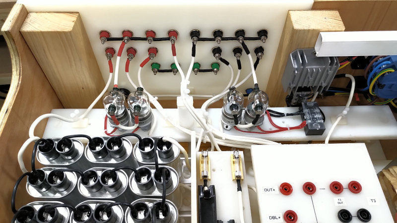
High Tension Output Panel
Fig 2.12 shows the HT Output panel in detail. The HT+ and HT- are each connected rails which form the final high voltage or high tension outputs. The various internal modules, OUT, RCT, and DBL can be connected to the output rails using HV jumpers. The left over terminals on each rail is then very convenient for the connection of the experiment, HV capacitors, measurement probes etc. The CAP1 and CAP2 connections are provided to conveniently connect series chains of HV capacitors providing safe and intermediate connection points in the chain. The output panel also has 4mm socket and heavy-duty terminal for the transformer earth to allow experiments to be referenced directly to the floated or connected transformer earth. This panel is the only one made in nylon to prevent any leakage or discharge between module terminals and outputs when used up to the maximum 18kV open circuit condition from 3 series transformers connected to the level shifter.
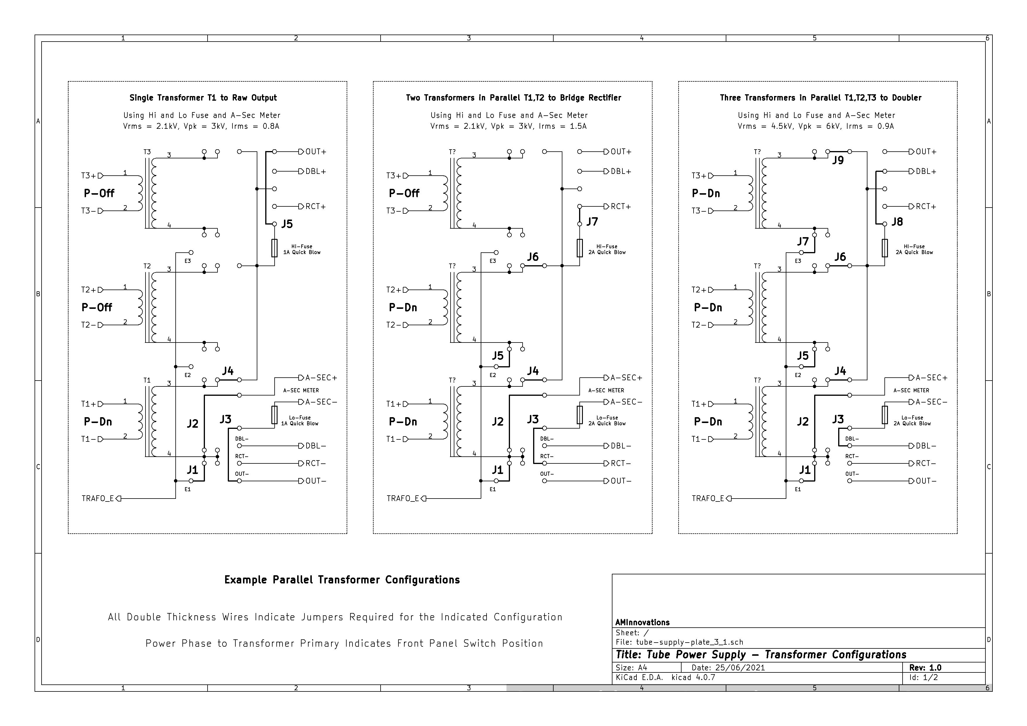
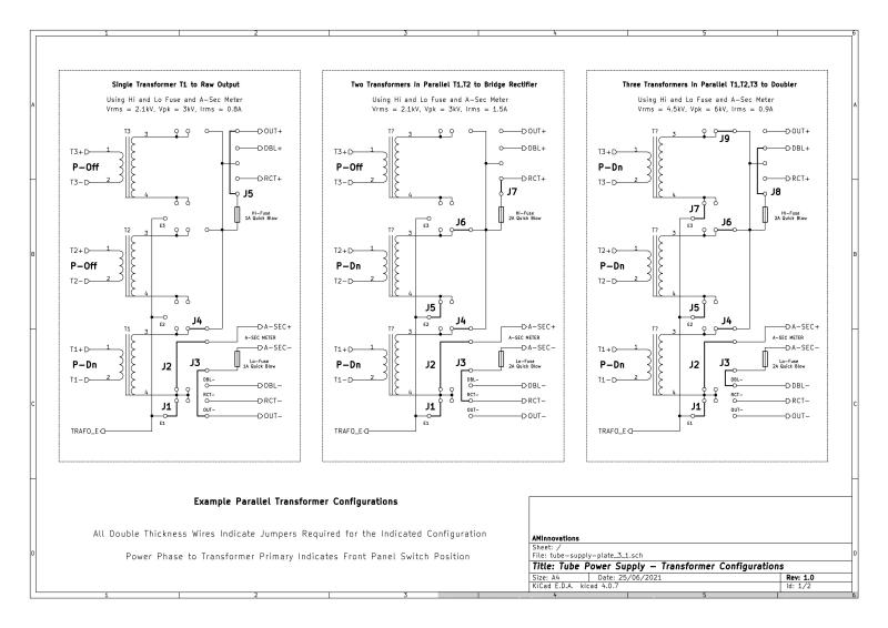
Figures 4 below show the example transformer connection diagrams to setup the supply into different configurations. I have selected a range of the most useful parallel and series setups, and which also configures the supply over its full range of voltage, current, and power output. The high-resolution versions can be viewed by clicking on the following links Fig 4.1, and Fig 4.2.
Fig. 4.1 Tube High Voltage & Plate Supply schematic showing examples of the jumper setup using the patch board for parallel transformer configurations, and connected to the internal HV bridge rectifier and doubler.
Fig. 4.2 Tube High Voltage & Plate Supply schematic showing examples of the jumper setup using the patch board for series transformer configurations, and connected to the internal HV bridge rectifier and doubler.
General Setup
In the final few sections of this post we look in more detail to the internal configuration of the plate supply using the transformer patch board, and the HT output rear panel. Any configuration of this supply must consider the requirements of the generator and experiment in terms of the required maximum voltage, current , and total power both real and reactive that will be drawn from the supply under different operating conditions e.g. varying tuning, matching, and output loading. With this established then the most simple, reliable, and optimal supply configuration can be arranged by setting up correctly the internal jumpers of the supply in order to meet the output requirements.
For example in the case of the GU-5B Armstrong oscillator coil unit used in the Wheelwork of Nature series, the nominal maximum plate potential is ~5kV. The CW power rated output when suitably cooled and driven around 1-5Mc for this tube is ~2.5kW, so at 5kV and 2.5kW of power the anode current could reach as high 0.5A. Considering current surges during extreme tuning experiments the anode current could reach considerably higher levels for very short time periods. The grid bias to keep the GU-5B oscillating under these conditions will need to be in the order of ~ 100mA – 500mA and can be adjusted using the grid bias rheostat for optimum drive matching to the experiment. Taking all this into consideration 2 series transformers will reliably supply ~ 4.2kV @ 0.8A, and up to 6kV open circuit, and 2 parallel transformers combined with the level shifter would provide ~ 4.5kV @ 0.6A, and again up to 6kV open circuit. For simplicity here I would use the 2 series transformers which also gives a better current rating, and less dissipated power with fewer HV components (less to go wrong) in the overall setup.
Now empirically the GU-5B can withstand substantially higher plate voltages when the generator is driven in low duty cycle pulsed mode, or using a staccato controller in the vacuum tube cathode connection. The advantage of this extreme operating condition is that the considerably increased anode potential will also considerably increase the peak-to-peak oscillation across the primary coil, which in turn will considerably increase the voltage magnification along the secondary coil, ultimately leading to much longer discharge streamers from the top-end of the Tesla coil secondary.
Under these operating conditions the plate supply could be as high as 9kV, and this would be best supplied by 2 series transformers with the level shifter which can supply up to 9.5kV @ 0.3A. In this extreme operating condition care needs to be taken not to allow the GU-5B to stop oscillating at full input voltage and power from the plate supply, as the tube anode would then be exposed to an open circuit voltage of almost 12kV which is too high for the GU-5B under any circumstances and could easily lead to anode-grid breakdown and destruction of the vacuum tube. Extreme operating conditions such as this have to be handled extremely carefully and with experience, but are discussed here to illustrate the setup of the plate supply necessary to operate in this region.
The other important consideration for the generator and experiment is the voltage envelope or driving waveform that is provided by the plate supply. For example the characteristics of a Tesla coil can vary enormously when the generator is driven by a sinusoidal, pulsed, chopped, or rectified and smoothed high voltage waveform. A setup consideration for the plate supply is whether to drive directly with the raw transformer output, use a rectified output with or without a tank/blocking/smoothing capacitor, or an output that is a continuous sinusoidal or chopped by an SCR. My own preference for these selections are as follows, but do very much depend on the type of generator being driven e.g. spark gap or vacuum tube, and the type of Tesla coil and phenomena that the experiment is working with e.g. Tesla’s Radiant Energy and Matter, Transference of Electric Power – Part 1, Single Wire Currents etc.
1. For experiments and generators in CW mode e.g. The Wheelwork of Nature – Fractal “Fern” Discharges, and High-Efficiency Transference of Electric Power, I use the bridge rectifier module with a tank/blocking capacitor as this allows for maximum power output efficiency from utilising both half-cycles of the transformer output, and also creates a positive forward pressure or positive voltage envelope. With a large tank/smoothing capacitor this makes for a very steady DC level anode supply which will result in high currents and hence strong, hot discharge phenomena, from powerful oscillations in the primary circuit. The blocking capacitor protects the semiconductor rectifiers from spikes and reflected power surges and transients.
2. For experiments and generators using spark gaps, or vacuum tubes in pulsed mode using a staccato interrupter, or other triggered grid devices e.g. Transference of Electric Power – Part 2, I prefer to use the raw output of the transformers in either parallel or series connection. The burst nature of the output especially with the SCR power control leads to enhancement of the non-linear and impulse like phenomena, and the setup of the pulsed triggering and staccato phasing is easier when matched to a positive or negative half-cycle envelope. This configuration is very robust for extreme operating, tuning and matching, as only the transformers are exposed to the raw output. MOTs are extremely robust provided they are not allowed to excessively overheat or are exposed to excessive series connected voltages.
3. For experiments requiring very high potentials such as Thyratron pulse generators, tank capacitor charging for impulse discharge experiments e.g. Displacement of Electric Power, I use the 2 series or 3 series configuration with the level shifter. These are specialised configurations which generate very high potentials at considerable output power, and requires considerable care and experience to operate safely. I will be covering specialised Thyratron generator usage and experiments using this plate supply in subsequent posts, but is noted here for completeness of the overall operating range and characteristics of this supply.
Parallel Transformer Setup
Fig 4.1 shows the circuit diagram configurations for the transformer patch board for parallel connection of the HV transformers. All the parallel arrangements rely on the core of the transformers being connected to Trafo earth (TRAFO_E). This connects all of the bottom ends of the transformer secondaries, the cores, together. The top-end of the secondaries are also connected together via jumpers that connect to the common positive output rail. From the common positive output rail, which includes the high-end protection fuse, a jumper connects to the raw output OUT+, the HV bridge rectifier RCT+, or the level shifter DBL+. The low-side of the connected secondaries are first connected via the low-end protection fuse through the secondary AC analogue meter and then to the negative output terminal fpr the selected output OUT-, RCT-, or DBL-.
In parallel modes it is normal to connect Trafo earth to the line supply earth via the jumper on the line supply power input panel on the rear of the plate supply. This effectively grounds the cores of the transformers to line earth and would be considered the safest configuration for running the HV supply at high output powers. However, if the generator or experiment creates considerable non-linear transients or impulses these can be passed back through to the transformers, even with a large blocking capacitor, and via the core connected secondary through to the line supply earth, and hence interfere or disturb the normal operation of other unprotected electrical equipment and instruments connected to the line earth. In this case it is sometimes necessary to remove the jumper between the Trafo earth and the line supply earth, isolating the transformers from the line supply earth.
Series Transformer Setup
Fig 4.2 shows the circuit diagram configurations for the transformer patch board for series connection of the HV transformers. In the series configurations the transformers rely on the fact that the cores are floating due to physical mounting on a nylon board. So the top-end of the T1 secondary will connect to the bottom-end of the T2 secondary or the core, with the top-end of the T2 secondary forming the high-side positive output, and the core of T1 forming the low-side output. In this 2 series transformer configuration the core of T1 can safely be connected to Trafo earth and hence the line supply earth with same considerations as in the previous section. It is important to not that the core or low-side of T2 is NOT connected to the Trafo earth, as it is in series with T1 and hence the T2 core ONLY connects to the high-side output of T1. Connection to the positive output rail, high-side and low-side protection fuses, and the output modules OUT, RCT, and DBL are the same as for the parallel connections in the previous section.
The case of 3 series transformers is a special one and needs more careful consideration. When the core of a MOT is connected to line earth as it would be in its normal primary use in a microwave oven, the potential difference between the core and the primary is only the line supply voltage, and the potential difference between the core and the secondary high-end is the maximum rated output of the transformer which is normally ~ 2.1-2.3kVRMS. The normal construction of a traditional MOT makes sure that both the primary and secondary coils are adequately insulated from the core and any magnetic shunts, according to their specific purpose, which is usually accomplished with resin impregnated and sealed cardboard or a form of thin plastic insulation kept in place again with resin.
In the case of unearthed cores in series arrangements the cores are now biased to potentials well above the primary line supply, and in this case we rely on the insulation of the primary and secondary coils from the core. In a 2 series transformer arrangement at maximum output the core of T1 is at line supply earth or for example 0V which creates no problem for the T1 primary coil, and the T2 core is at ~ 2.1kV which also does not present a problem for most good condition MOTs. The high-end of the T2 secondary is then at ~ 4.2kV, the differential across T2 again only being ~ 2.1kV. In this way the 2 series transformer arrangement can be used safely and stably without breakdown between the core and the secondary, or the core and the primary. Open circuit without a load the core of T1 will be at ~ 3kV and the output at almost 6kV which is also ok for this arrangement, as MOT design covers the open circuit fault condition in a microwave oven.
This would not be the case for a 3 series transformer arrangement where T3 was simply added on top of the 2 series setup. Now the core of T3 would sit at ~ 4.2kV and the high-end of T3 at ~6.3kV, and this is under maximum output and full load. Open circuit the core of T3 would sit at ~ 6kV and the output at almost 9kV. The 4.2 – 6kV potential of the T3 core is too much potential difference between the primary coil and the core. The windings of the primary coil in T3 are still at the line supply voltage level, and most MOT insulation will fail when exposed to this 6kV potential difference, resulting in strong breakdown between the core and primary, and in some cases the secondary and core, and this is for a good condition transformer.
To use 3 series transformers safely and reliably the Trafo earth must be moved to the midpoint of T1 and T2 so that the T1 core and the T2 core are connected to Trafo earth and hence line supply earth. Now the phase of the line supply is adjusted for T1 and T2 to be in anti-phase to each other (via the front-panel transformer switches), and so the T1 high-end of the secondary goes negative -2.1kV and the high-end of T2 goes positive +2.1kV, the potential difference across the two transformer outputs being again ~4.2kV. Now T3 can be added on top of the T2 output in series with the T3 core sitting at 2.1kV fully loaded, and 3kV open circuit. The T3 phasing of the primary is set to the same as T2, and opposite to T1. Now 3 series transformers can produce a loaded output potential difference of 6.3kV, and ~ 9kV open circuit, without breakdown between the core and the primary coils at the line supply.
In relation to Trafo earth or line supply earth if connected, then T1 high-side is at -2.1kV or -3kV OC, T2 high-side is at +2.1kV or +3kV OC, and T3 high-side is at +4.2kV or +6kV OC. In this configuration the negative side output of the power supply is now NOT earth, which is very important when connecting the vacuum tube generator. The negative rail is now -2.1kV and hence both the generator and the experiment must use the negative rail as the bottom-end or base connection for the various units, and NOT the line supply earth. To connect the generator and experiment to line supply earth at the bottom-end would be to short the output of transformer T1, which will throw-out the MCB at sufficiently high input current.
Operation, Line Supply and Safety
Operation of a high voltage high power supply like this one should always be undertaken with great care and caution and with well defined method that is adhered to throughout its operation. Establishing a good operation procedure introduces a disciplined approach, and reduces the chances of unexpected events and mishaps arising from careless use. Remember that a high voltage supply is instantly lethal if not used correctly. What follows here are some of my own procedures when working with this type of high voltage supply:
1. Always where possible operate the supply using the remote control at a reasonable distance from the high voltage supply.
2. When approaching the high voltage supply always check the V-OUT meter is on zero, and if not use the discharge control on the remote control.
3. When setting up the power supply configuration using the transformer patch board, or adjusting any internal part of the supply, make sure that the line supply is turned-off at the primary line supply input panel at the rear, and that any capacitive elements in the system are discharged.
4. Always test a new configuration of the supply at very low input power, to check that setup has been accomplished correctly.
5. When tuning an experiment always run the high voltage power supply at low output power until the correct operating point has been found.
6. Wind up the power to an experiment slowly, restricting high power operating to short bursts until satisfied that the supply, generator, and experiment are stable and can withstand longer sustained high power operation.
7. For sustained high power operation turn on the cooling fans, and preferably close the supply top panel in order to improve the cooling efficiency. During long periods of experimentation at high-power allow the system to cool intermittently, and do not allow the transformers cores to become overheated.
8. If a protection fuse is blown, disconnect the generator and experiment and safely investigate the reason and source of the fault event.
9. Never rush to change the power supply setup, and never leave the power supply operating unattended.
10. Arrange if possible a single master emergency power-off switch which will cut all power to the supply, and if the experiment produces phenomena with strong dielectric and magnetic induction fields consider wearing appropriate protective gear.
Adhering to these kind of safety procuedures in setup and operation are critical when working in high voltage research and development. The supply presented here is robust, and with a very wide range of output performance, and when used safely and correctly with suitable generators and experiments, is capable of covering the wide range of phenomena generally accessible in the alternative electricity research field, with power levels up to 5kW.
Another module in the tube power supply series is a heavy-duty line supply filter and power factor correction unit. This module which attaches between the line supply and power input rear panel, performs two important jobs. The first is to isolate the line supply from higher frequency transient noise coming back through the experiment, generator, and plate supply, which is important if the experimental apparatus is setup in a domestic setting, or close to any other more sensitive electrical equipment such as computers and digital communications equipment etc. My research lab is arranged in a rural industrial environment that caters for a lot of welding, and other electrical disturbance processes and apparatus, and hence the short run electrical disturbance created by my Tesla coil experiments does not disturb other endeavours or power supply users.
The second job is to correct the low power factor that arises from running microwave oven transformers. The very high inductive load of a MOT, and especially multiple MOTs driven either in parallel or series configurations easily reduce the power factor to ~ 0.6 or even down as low as ~ 0.4. This is not ideal for longer term high power experiments where the input currents can become very high and the overall apparent input powers can rise as high 10kVA when using all three transformers flat-out. Power correction using parallel connected PFC capacitors is accomplished by this module and uses a range of jumper selectable capacitors to improve the power factor during longer experimental runs. Overall the actual running time of a Tesla coil in a research environment is usually limited to short run bursts, and hence the impact on the line supply in the correct industrial setting is minimal. This line supply module will be covered in detail in a subsequent post.
Summary
Overall the 5kW high voltage and plate supply presented in this post is very robust, is easily configured to a wide range of different output voltage and power levels, and is also relatively straightforward to operate with the necessary experience and know-how. This supply is intended for an electricity research and development environment using Tesla coils and associated generators, and in a non-commercial and non-industrial setting. This power supply will feature in quite a few of the experiments yet to be presented on this website, which will also show more detail as to the setup, usage, and operating characteristics of the complete tube power supply series.
The next parts in this tube power supply series will cover the individual tube board designs and configurations for parallel and push-pull tube operation, and also pulsed power using a staccato interrupter.
1. A & P Electronic Media, AMInnovations by Adrian Marsh, 2019, EMediaPress
2. Dollard, E. and Energetic Forum Members, Energetic Forum, 2008 onwards.
In this follow up experiment in the Wheelwork of Nature series we take a look at vibration, frequency, and discharge form that results from a set of Tesla coils designed to cover an operating frequency range between 300kc and 4Mc. If you have not done so already I recommend reading or reviewing the first experiment in this series The Wheelwork of Nature – Fractal “Fern” Discharges, which will set the basis for this current experiment. In the original experiment a range of experimental variations were tested in order to identify the origin of the fractal “Fern” discharge form, which is a distinct and significant departure from the discharge form normally observed in Tesla coils constructed using a basic standard design format, and constructed with readily available materials and processes. Variations to the experiment included, changing the matching and tuning of the Tesla coil, the excited resonant mode, the generator waveform, the type of vacuum tube used as a generator, and a top-load on the Tesla coil. The only significant variation to the discharge form was noted between the upper and lower parallel resonant modes of the Tesla coil, and hence it was concluded that frequency, or more correctly vibration, of the Tesla secondary coil was key to the nature and form of the fractal “fern” discharge.
The original coil was theoretically designed with a series resonant mode frequency of the secondary ƒSS ~ 3.5Mc in the 80m amateur radio band, and was subsequently measured using a vector network analyser to have a series fed fundamental resonant frequency ƒSS = 3.44Mc. When this was combined with a primary coil and RF ground it was found to reduce to ~ 3.18Mc. The upper and lower parallel resonant modes were found to be around 2.7Mc and 3.4Mc. The generator used was a basic class-C Armstrong oscillator using a single GU5B vacuum tube, and dual 883C vacuum tubes in the variation generator. This form of generator will oscillate readily at the upper or lower resonant parallel modes and can be tuned over a frequency band using a vacuum variable capacitor as a parallel tank capacitor in the primary circuit. This gave a tuned range from low end of the lower parallel mode at ~ 2.4Mc to the high end of the upper parallel mode at ~ 3.6Mc. Across this entire tuned range the discharge form was the fractal “fern”. The only significant variation was at the upper parallel mode, where the fractal “fern” appeared more compact, tightly formed, and with more dense secondary and tertiary tendrils.
In this next experiment the exploration of vibration and frequency is extended across a much wider range by using a set of Tesla coils that are designed on the same geometry, with the same materials, but with different wire type and gauge, and hence the fundamental series resonant mode changes with the wire length. Originally five coils were designed and constructed, with series resonant mode frequencies of ƒSS ~ 357kc, 570kc, 1013kc, 2068kc, and the original at 3494kc. The general design characteristics of the coils, key measured, operating and tuning characteristics are summarised in figures 1 shown below, and explained in detail later in this post.
In practise, when using a self-tuned feedback oscillator as the generator, the lower frequency coils tend to preferentially oscillate at the 2nd or 3rd harmonic frequency around 1Mc, where the gain of the vacuum tube generator is higher, and the capacitive loading in the primary is lower. Increasing the tank capacitance to tune the fundamental of these lower frequency coils, significantly capacitively loads the vacuum tube generator reducing the Q of the system dramatically, and making it very difficult to oscillate in class-C mode. Ideally the two lowest frequency coils would be driven directly at the series resonant mode frequency ƒSS, however this drive strategy is not best suited to the scope of this experiment where variable frequency adjustment during operation is preferred. As a result of this, and without wanting to significantly change the generator and matching for this experiment from the previous one, the three upper frequency coils only are demonstrated in the video for this experiment. In practise that proved to be more than adequate to demonstrate the transition of the discharge form, from the fractal “fern” discharge, to the more standard “swords” form, which is commonly observed for a standard Tesla coil design when driven by a vacuum tube generator.
The video experiment demonstrates and includes aspects of the following:
1. Three secondary coils based on the same geometry, dimensions, and construction, with different wire gauge and hence wire length, producing a different fundamental series resonant frequency in each secondary coil.
2. A standard vacuum tube Tesla coil generator (VTTC), operated in CW mode using a pair of 833C vacuum tubes (VT) arranged in parallel as a tuneable class-C Armstrong oscillator.
3. The tube power supply (HV & Plate) configured for 2 series transformers with a nominal output of 4.2kV @ 0.8A, 3.3kVA, HV bridge rectified, and with 25nF 25kV blocking capacitor at the output, and operated up to 3kW line input power.
4. Secondary coils with nominal fundamental series resonant frequencies of ~ 3.5Mc, 2.0Mc, and 1Mc, could be easily exchanged, tuned, and matched to the VT generator.
5. The 3.5Mc coil operated over a range of 2.4-3.3Mc, shows the fractal “fern” discharge over the entire frequency band. A tighter and denser fractal “fern” was observed across the upper parallel mode.
6. The 2.0Mc coil operated over a range from 1.5-2.3Mc, shows the fractal “fern” discharge at the upper parallel mode, and the “swords” discharge at the lower parallel mode.
7. The 1.0Mc coil operated over a range from 970kc-1.4Mc, shows the “swords” discharge over the entire frequency band.
8. The transition from fractal “fern” to “swords” occurs between 1.8-2.0Mc, where the “sword” discharge retains slight curvature until frequencies < 1.5Mc.
9. Conjecture that the variation of discharge form may result from the changing vibrational qualities within the relationship between the dielectric and magnetic fields of induction at different frequencies, and hence part of the underlying principles and mechanisms within the Wheelwork of Nature.
Principle of Operation and Construction of the Experimental System
The experimental apparatus uses the same high voltage plate tube supply from the pervious experiment, configured in the same way with two series transformers, bridge rectified, and with a 25nF blocking capacitor at the generator output to protect the semiconductors of the bridge rectifier. The design, construction, and operation of this high voltage tube supply is covered here Tube Power Supply – High Voltage & Plate. The generator itself uses the dual 833C tube board with the tube supply heater unit as an class-C Armstrong oscillator, both of which were used in the variation experiments in the first part of this series, and are covered in detail in Tube Power Supply – Heater, Grid & Screen. The dual 833C tubes proved to be more flexible over a wider frequency band than the single GU5B based generator used in the primary Wheelwork of Nature experiment. The principle of operation of the generator, setup, operating characteristics, and schematic are covered in detail in the original post here The Wheelwork of Nature – Fractal “Fern” Discharges.
The feedback coil for the Armstrong oscillator now has variable windings, and is positioned offset from the secondary coil. The variable turn geometry of the feedback coil facilitates more accurate and optimal tuning of the generator based on the secondary coil used, and the lower or upper parallel mode being explored. Too much feedback to the generator will distort the drive waveform away from a clean sinusoidal, and too little feedback makes the oscillation unstable, and with a reduced gain in the generator. The optimal adjustment was to establish oscillation with the maximum number of turns on the feedback coil which produced a clean sinusoidal oscillation in the primary tank circuit. The number of turns varied for each secondary coil, and for the upper or lower parallel mode for each coil. With the correct number of turns set on the feedback coil, the generator match to the experiment was fine adjusted using the grid bias rheostat to produce maximum output from the secondary, with minimum average grid current.
Figures 2 below show a range of pictures of the experimental apparatus used in the video experiment, along with the measurement equipment, and some of the key construction details that vary from the original experiment.
Fig. 2.1 The five different frequency Tesla secondary coils are the same geometry and construction materials, but wound with a different guage of wire. The wire length of each coil is different and hence its series fundamental resonant frequency is also different.
Fig. 2.2 The complete experimental setup showing the coil unit with external adjustable feedback coil and interchangeable secondary coil, the dual 833C tube supply heater and grid unit, the high voltage tube plate supply, and the measurement instrument rack.
Fig. 2.3 The adjustable feedback coil for the Armstrong oscillator has individual tap points on the coil for fine tuning of the feedback bias. This prevents tube under-drive and over-drive, and ensures a good clean sinusoidal oscillation from the generator to the primary coil.
Fig. 2.4 The KP1-4 10kV vacuum variable capacitor in the coil unit has a range from 20-1000pF and forms the variable tuning capacitor in the parallel resonant circuit with the primary coil. When driven at the upper or lower parallel resonant modes, the tuning capacitor can be used to adjust oscillation frequency during operation.
Fig. 2.5 The primary coil is a new design using 12 AWG silicone-coated, micro-stranded, cable wound on a former with posts to minimise over-heating. Here the vacuum variable capacitor is shunted with a 1000pF doorknob, giving an adjustment range of ~ 1000-2000pF for the 1Mc secondary coil.
Fig. 2.6 The dual 833C force-cooled generator is here used as a class-C Armstrong oscillator throughout the experiment. This generator is exceedingly robust and powerful with plate voltages up to ~ 5kV and total sustained output power in the region of 2.5kW. The grid leakage bias is fine tuned using the 150W rheostat and the number of feedback coil turns.
Fig. 2.7 The DG8SAQ vector network analyser here being used to measure the series fed resonant frequency and harmonics of the secondary coil. This measurement technique allows for accurate characterisation of the secondary coil properties, and when combined with the primary coil a good measure of the required matching and hence driven point of the Tesla coil.
Fig. 2.8 The high voltage plate supply is configured for two transformers in series, with the bridge rectifier output, giving ~ 4.2kV @ 0.8A maximum output. The blocking capacitor at the HV output is a 25nF 25kV pulse capacitor to prevent transients and high frequency oscillations from the experiment being reflected back into the power supply.
Fig. 2.9 When combined with the primary coil and tuned to balance the upper and lower parallel modes, the impedance characteristics of the Tesla coil show, from the perspective of the generator, the upper and lower frequency bands that the system can be driven over.
Fig. 2.10 A variable capacitance box was used to accurately determine the primary circuit capacitance necessary to balance the upper and parallel resonant modes. Here the lowest frequency coil required in the region of 12.5nF to balance the parallel modes. The capacitance box is removed before operation and replaced with suitable HV capacitors.
Figures 3 below show some of the operation highlights during the experimental running, and the typical output from the measurement equipment, including generator driving frequency and waveform.
Fig. 2.1 Running operation with Tesla coil 1 at the lower parallel mode at 2.71Mc 2.0kW, showing a strong and well defined fractal "fern" discharge extending over 30cm from the breakout point.
Fig. 2.2 Running operation with Tesla coil 1 at the upper parallel mode at 3.20Mc 1.8kW, showing a tighter and more densely packed fractal "fern" discharge, which also takes on the more regular appearance of a "ball" with a "fern" stucture within it.
Fig. 2.3 Running again with Tesla coil 1 at the lower parallel mode at 2.71Mc 2.0kW, showing the spectacular double twisted fractal "fern" discharge. This is where two primary streamers are tightly wound around each other, and extend over 30cm from the breakout point.
Fig. 2.4 Large primary streamers with many secondary and tertiary tendrils make for a spectacular discharge pattern. The dual 833C tubes can be seen running with a healthy red-glow on the plates, and with 2kW of input power supplied by the high voltage plate supply.
Fig. 2.5 The experimental apparatus consisting of the coil unit (Tesla coil only), the tube supply heater and grid/screen unit, with the dual 833C tube board installed as a class-C Armstrong oscillator, and the tube supply high voltage unit configured with 2-series transformers and the HV bridge rectifier, and a 25kV 25nF blocking capacitor at the HT output.
Fig. 2.6 The experimental operation is measured and monitored using the lab mobile measurement equipment. This mostly consists of HP and Tektronix test equipment from the 1970s-90s era, which run very stably and reliably in the close presence of a Tesla coil or TMT system, running at moderately high output powers. More modern test equipment often has significant issues running reliably in the harsh electromagnetic environment of Tesla based research.
Fig. 2.7 In this measurement the oscillation waveform of the secondary coil is being monitored on HP54542C oscilloscope, and the frequency of this oscillation at 2.746Mc being measured using the Teltronix DC504 frequency counter. Both instruments are very stable under these conditions. The oscilloscope shows a well defined sinusoidal waveform indicative of a well matched and tuned generator, driving a clean oscillation at the lower parallel mode of coil 1.
Again Tccad 2.0 was used for a rapid and approximate indication of the electrical and resonant characteristics of the secondary coils, the detailed results of which are shown below in figure 4. The wire selected for coil 1 and 2 is a good quality silicone coated multi-stranded conductor, the silicone coating being very good both thermally, and as an insulator to prevent breakouts and breakdown from the upper turns of the coil to the lower ones. For secondary coils 3, 4, and 5, a good quality polyester-polyamide coated magnet wire was used, with the final wound coil being further coated with high-temperature lacquer. The final lacquer coating is used to keep the windings in place, and add some additional breakdown insulation protection.
Fig. 4.1 Tccad Coil 1 = 3494kc.
Fig. 4.2 Tccad Coil 2 = 2068kc.
Fig. 4.3 Tccad Coil 3 ~ 1013kc.
Fig. 4.4 Tccad Coil 4 ~ 570kc.
Fig. 4.5 Tccad Coil 5 ~ 356kc.
Small Signal AC Input Impedance Measurements
The small signal ac input impedance Z11 for each Tesla coil was measured directly using an SDR-Kits VNWA vector network analyser, as used on many experimental pages on this site. Figures 5 show the series-fed free resonant characteristics of the five Tesla secondary coils.
Fig. 5.1 Series-fed coil 1 with series mode fss = 3.41Mc @ M1, and parallel mode fsp = 4.26Mc @ M2.
Fig. 5.2 Series-fed coil 2 with series mode fss = 2.03Mc @ M1, and parallel mode fsp = 2.52Mc @ M2.
Fig. 5.3 Series-fed coil 3 with fundamental series mode fss = 1.10Mc @ M1, and parallel mode fsp = 1.37Mc @ M2. 2nd, 3rd, and 4th odd harmonics are also present in the scan.
Fig. 5.4 Series-fed coil 4 with fundamental series mode fss = 0.64Mc @ M1, and parallel mode fsp = 0.80Mc @ M2. 2nd to 7th odd harmonics are also present in the scan.
Fig. 5.5 Series-fed coil 5 with fundamental series mode fss = 0.41Mc @ M1, and parallel mode fsp = 0.52Mc @ M2. 2nd to 12th odd harmonics are also present in the scan.
To view the large images in a new window whilst reading the explanations click on the figure numbers below.
Fig 5.1. Shows the series fed input impedance Z11 for Tesla coil 1, design ƒSS = 3.49Mc. The measured fundamental series resonant mode ƒSS @ marker M1 = 3.41Mc, and with a 1m single wire extension at the bottom-end of the negative terminal of the VNWA. The parallel mode ƒSP @ M2 = 4.26Mc, and is characteristic of a standard Tesla coil design where the parallel mode is above the series mode when the secondary is on its own in a series-fed configuration. The characteristics of Tesla coil and TMT input impedance Z11 is covered in detail here Cylindrical Coil Input Impedance – TC and TMT Z11. The large and well defined phase change at M1 shows the high quality factor Q of the coil, which mostly occurs when the geometry of the turns of the coil are not too tight, and have adequate spacing between them, in this case the distance between turns is ~ 1.35mm, the thickness of the silicone wire cladding, and the diameter of the wire is ~ 1.1mm. Geometry of Tesla coils and there design is covered in detail here Tesla Coil Geometry and Cylindrical Coil Design.
The coil is purely resistive at both the resonant modes ƒSS and ƒSP. At the series mode ƒSS reaches a minimum at ~ 70Ω, and a maximum of ~ 80kΩ at the parallel mode ƒSP. Both series and parallel modes are particularly useful depending on what type of generator is being used to excite the Tesla coil. A tuned linear amplifier, spark gap generator, or solid state inverter are best suited to driving the series mode, and a series feedback oscillator such as a class-C Armstrong oscillator is suited to drive at the parallel mode. With correct matching and tuning it is possible to couple significant power into the Tesla coil through either the series or parallel modes. The parallel mode allows for frequency adjustment dependent on how the tank circuit in the primary is setup, which is particularly useful for this experiment where a range of frequencies can be tuned dynamically during operation using a vacuum variable capacitor. If secondary feedback is arranged through a pick-up coil to the vacuum tube generator the parallel mode can be tracked dynamically with little additional tuning required during operation, other than at the band-edges where the grid-bias will need adjusting, and the feedback coil turns optimised.
At the series mode, frequency can also be adjusted by changing the wire-length at the top-end of the secondary coil. This is best affected using a telescopic aerial or other adjustable wire length, but is not so practical to adjust during operation without re-tuning the generator to the new frequency. Driven either at the series mode or the parallel mode, transmission mode conversion can be accomplished between the driving primary circuit, and the cavity of the secondary coil formed with the single-wire or transmission medium connected to the bottom-end of the secondary coil. In principle, power in the TEM transmission mode in the primary circuit, can be transferred and transformed to the LMD transmission mode in the cavity of the secondary coil. The cavity in principle can be made to extend over very large distances, presenting the possibility for power transfer at very low-loss over very large distances in the far-field, and many times the wavelength of excitation at the generator. A second tuned Tesla coil in the cavity of a TMT system transforms the LMD mode back to the TEM mode in the receiver primary. The transfer of power, which accompanies the transformation of transmission mode from the cavity in the secondary to the primary circuit of the receiver, can then be used to do work in the load. It is interesting to note that the frequency of the LMD mode in the cavity is not the same as the frequency of the TEM modes in the primary of the transmitter and receiver.
Fig 5.2. Here secondary coil 2 has series mode ƒSS = 2.03Mc, and parallel mode ƒSP = 2.52Mc. Compared to coil 1 this is more tightly wound, with reduced conductor spacing and more turns, and hence the Q has reduced significantly, as can be seen in the reduction of the magnitude of the phase swing at M1. Both coils 1 and 2 are on the same magnitude and phase scales, and the phase reduction for this coil is a factor of ~ 2. The longer wire length has also considerably increased the coil resistance at the series and parallel modes, RSS = 160Ω, and RSP = 122kΩ. The second odd harmonic at 3λ/4 is just visible at M3 @ 4.97Mc. This coil when combined with the primary in the video experiment shows the transition between the upper parallel mode and the fractal “fern” discharge, and the lower parallel mode which shows the “swords” discharge with an additional slight curvature. However, in the series-fed Z11 small signal impedance analysis there is nothing obvious that suggests some different electrical characteristic or feature that may be responsible for this dramatic transition from one discharge form to the other. It is worth considering at this point as to whether interaction between harmonics has any bearing on the discharge form. As the fundamental resonant frequency goes down through designed wire-length the harmonic frequencies become progressively closer which makes it more possible for energy to be transferred between the harmonics through the non-linear nature of the discharge.
Fig 5.3. Shows secondary coil 3 and the final coil used in the video experiment. Here the 2nd, 3rd, and 4th odd harmonics are very clearly defined. The phase scale has been expanded from 20°/div to 10°/div to show clearly the phase swing as it collapses with reducing Q of the coil, much reduced wire spacing, increased turns, and hence increased series coil resistance. Operation of this coil was still at the fundamental resonant modes rather than at harmonics, and when combined with the primary, (shown in figures 6), result in the parallel mode operating points used in the video. The series mode ƒSS = 1.10Mc with RSS ~ 370Ω @ M1, and the parallel mode ƒSP = 1.37Mc with RSS ~ 191kΩ @ M2. Harmonic frequencies extend at nλ/4 where n is an odd number, and with progressively reducing Q, and hence have a smaller and smaller impact as frequency increases. This coil clearly displayed the straight “swords” discharge at both the upper and lower parallel modes of operation, the slight curve was no-longer present and each discharge streamer projected straight outwards from the breakout point at the top-end of the coil. Streamers continued to be white and “hot” consistent with the generator drive which is at a maximum capped voltage defined by the two series transformers driven by the SCR, and current rich controlled by the “on” phase of the SCR power control.
Fig 5.4. and 5.5. Show the two lower frequency coils 4 and 5 that were not demonstrated in the video experiment. In both Z11 measurements there are a very large number of harmonics, and the phase scale has been expanded again from 10°/div to 5°/div to reflect the collapsing Q of the coils, the rapidly rising series resistance from thinner gauge wire of many turns, and hence much longer wire lengths. Lower frequency Tesla coils like these tend to oscillate at a harmonic frequency when driven by a feedback oscillator using the parallel mode resonant frequency. In Fig. 5.4 it can be seen that the Q of the second odd harmonic at M3 is actually higher than the fundamental at M1. In this case the coil is more likely to stably oscillate at ƒSP2 the second harmonic parallel mode when driven using a series feedback oscillator. This will become clearer when we look at the parallel mode points when combined with the primary in figures 6.
Consequently many lower-frequency standard Tesla coils presented on the Internet tend to oscillate stably at the 2nd or 3rd harmonic when driven by a series feedback oscillator. To drive these two coils at their series fundamental resonant modes a fixed frequency linear oscillator or amplifier needs to be used where the frequency can be selected and fixed, and the generator is specifically matched at this fixed frequency, and then considerable power can be stably transferred to the secondary. This generator is more complicated than the series feedback tube oscillator, and required more setup, tuning, and matching to run at the equivalent power used in this experiment. For compatibility and simplicity with the previous Wheelwork of Nature experiment, I have kept the generator the same as before and avoided any additional complexity in the experiment, and its possible interpretation. I will look to make a video of these two low frequency coils driven by this form of fixed frequency generator in a subsequent experiment.
Figures 6 show the balanced parallel modes for each secondary coil when combined with the primary and tuned to balance using the primary circuit tank capacitor Cp. The primary tank capacitor is based on a KP1-4 10kV vacuum variable capacitor with range 20-1000pF. For the lower frequency secondary coils 3, 4, and 5, it was necessary to add a parallel static capacitor to the variable capacitor in order to increase the tank capacitive loading, and hence achieve balance of the upper and lower parallel modes.
Fig. 6.1 Balanced primary-fed coil 1. The series mode fo = 3.45Mc @ M2, and the parallel modes fl = 3.05Mc @ M1, and fu = 3.81Mc @ M3. Cp = 197pF to balance the parallel modes.
Fig. 6.2 Balanced primary-fed coil 2. The series mode fo = 2.06Mc @ M2, and the parallel modes fl = 1.85Mc @ M1, and fu = 2.31Mc @ M3. Cp = 529pF to balance the parallel modes.
Fig. 6.3 Balanced primary-fed coil 3. The series mode fo = 1.12Mc @ M2, and the parallel modes fl = 1.01Mc @ M1, and fu = 1.28Mc @ M3. Cp = 1634pF to balance the parallel modes. Interaction between the self-resonance series modes of the primary, and the second series harmonic of coil 3 occurs at 2.72Mc @ M4.
Fig. 6.4 Balanced primary-fed coil 4. The series mode fo = 0.65Mc @ M2, and the parallel modes fl = 0.58Mc @ M1, and fu = 0.73Mc @ M3. Cp = 4951pF to balance the parallel modes. Interaction between the self-resonance series modes of the primary, and the second series harmonic of coil 3 occurs at 1.59Mc @ M4.
Fig. 6.5 Balanced primary-fed coil 5. The series mode fo = 0.42Mc @ M2, and the parallel modes fl = 0.38Mc @ M1, and fu = 0.48kc @ M3. Cp = 11676pF to balance the parallel modes. Interaction between the self-resonance series modes of the primary, and the second series harmonic of coil 3 occurs at 1.04Mc @ M4.
To view the large images in a new window whilst reading the explanations click on the figure numbers below.
Fig 6.1. Here secondary coil 1 has been added to the primary circuit shown in Fig. 1.5. The primary tank circuit is formed by the primary coil, the vacuum variable capacitor, and any additional fixed loading capacitance. When tuned correctly the parallel mode from the secondary coil occurs at the same frequency as the parallel mode from the primary coil. When the coils are coupled energy is exchanged backwards and forwards between the two parallel modes which causes “beat” frequencies, and a frequency splitting of the two parallel modes. The degree of splitting depends primarily on the magnetic coupling coefficient k, the Q of the two coils, and the geometry of the coils. The parallel mode from the primary results from the self-resonance of the primary coil, which is typically for the coil shown, around 30-50Mc for the fundamental series mode. The parallel mode of this self-resonance is at a much lower frequency than the series mode, and can be tuned down to even lower frequencies by addition of CP, the primary circuit tuning capacitance. The splitting of the two parallel modes from the primary and secondary results in the lower and upper parallel resonant modes of the Tesla coil, and can be driven and tuned directly when using a series feedback oscillator type generator. Tesla coil resonance modes are covered in much more detail here Cylindrical Coil Input Impedance – TC and TMT Z11.
When the parallel modes are tuned using CP to a point where the magnitude of their impedance is equal, and the phase angle of their impedance is zero, then the balanced mode is achieved. This condition balances the two parallel modes of the Tesla coil either side of the series fundamental mode, and has been found in some cases to be an optimum driving condition for a Tesla coil for certain different types of phenomena including, High Efficiency Transference of Electric Power in the close mid-field region, balanced TMT setup for LMD transmission experiments in Transference of Electric Power, and the equilibrium initial condition for experiments in the Displacement of Electric Power. This typical balanced mode for a Tesla coil is shown in this figure, where the fundamental series resonant mode is at M2 @ 3.45Mc, and the lower and upper parallel modes are at M1 @ 3.05Mc, and M3 @ 3.81Mc, and the primary tank capacitance CP was set at 197pF to achieve this balanced point. At all of these three resonant modes the phase of the impedance is 0 degrees, showing the input impedance seen by the generator is entirely resistive, with no reactive components. The Tesla coil can be driven from any one of these three modes, and considerable power coupled intro the resonator from the generator.
Generator matching at any of these three modes requires an impedance transformation from the output impedance of the generator to the input of the Tesla coil, where at the three resonant modes this can be accomplished through a transformation of the resistive component only. For the series mode this usually involves using a tuning stage such as an high-power antenna tuner, specifically arranged balun or unun, or a fixed or variable RF transformer such as a “swing-link” tuning transformer. For example, to tune the series mode directly at M2, the input impedance Z11 is entirely resistive and RS = 28.5Ω. If a linear amplifier is being used as the generator with a usual output impedance of 50Ω, then an antenna tuner could be used to produce a good match with standing wave ratio (SWR) ~ 1. A 1:2 Balun (not 2:1) could also be used here since the ratio of the input resistance at M2 is close to 1:2. A balun is also useful here to convert the unbalanced coaxial feed of the generator to the balanced half-wave primary coil feed (λ/2). This considerably reduces radiated energy from the outer surface of the coax cable between the generator and Tesla coil, and also improves measurement accuracy when using inline RF power meters such as Bird Thruline analog 4410A, and digital 4391A.
For the parallel modes the input impedance is a much higher resistance e.g. at M1 = 3.05Mc, Rs ~ 10.7kΩ. This high impedance is very suitable for driving directly using the high plate impedance of a vacuum tube oscillator. When arranged properly at resonance so the match is purely resistive, or as close as can be accomplished, the match can be coarse adjusted through the number of feedback turns from a pickup coil placed close to the secondary coil. This type of positive feedback to the oscillator also means that the parallel mode frequency can be tracked by the oscillator, and hence a simple but highly effective tracking generator is arranged. By adjusting the position of the parallel modes, and which parallel mode is dominant, and hence the point of tracking, the generator can be auto-tuned over a wide frequency range either side of the series fundamental mode. Fine tuning of the match at any specific frequency is accomplished by adjusting the grid bias and/or the grid leakage at the grid storage circuit. If both of these are arranged with a rheostat very fine tuning and matching can be accomplished over a wide range of tracked frequencies. This particular generator arrangement has been very successfully used so far in the Wheelwork of Nature and Transference of Electric Power experimental series. It is relatively simple to arrange, is very tolerant to moderate mismatch conditions between the generator and the Tesla coil, and is highly flexible in its variable frequency range which can be adjusted directly during operation by adjustment of a vacuum variable capacitor.
When operated in the parallel mode using a feedback oscillator the tank capacitance CP was tuned either side of the 197pF necessary for the balanced point. At the balance point the oscillator output will not be stable as it jumps between the equal magnitude lower and upper parallel modes, and back again. For stable operation in the lower parallel mode CP is increased, and in the video experiment CP ~ 230pF was used to set the starting point of oscillation at 2.7Mc with the lower parallel mode impedance dominant. For stable operation in the upper parallel modes CP is reduced, and in the video experiment CP ~ 150pF was used to set the starting point of the oscillation at 3.2Mc with the upper parallel mode impedance dominant. The measurements taken in figures 6 are with the secondary coil connected to the experiment earth, that is, with the line earth of the apparatus only. When the experiment was further connected down to the RF earth for operation, the effective wire length increases slightly, and hence the fundamental series mode shifts down from ƒO = 3.45Mc to ƒO ~ 3.0Mc, the lower parallel mode ƒL ~ 2.8Mc, and the upper parallel mode ƒU ~ 3.1Mc which correspond with the operating frequencies presented during in the video experiment.
Fig 6.2. Here Tesla coil 2 has been balanced in the same way by increasing the primary tank capacitance to CP ~ 529pF, ƒO @ M2 = 2.06Mc, ƒL @ M1 = 1.85Mc, and ƒU @ M3 = 2.31Mc. The resistance of the two parallel modes have decreased significantly, mainly due to the additional capacitive loading in the primary, and also slightly from the lower frequency. The series mode resistance has also dropped from 28.5Ω @ 3.45Mc to 20.0Ω @ 2.06Mc. In this scan the series fundamental mode of the primary coil can just be seen at the very top-end of the scan at M4 = 4.98Mc. This also shows the wide frequency gap between the series mode of the primary coil self-resonance and the parallel mode, which is here balanced with the parallel mode of the secondary coil. As the primary tank capacitance is increased this series mode self-resonance of the primary coil moves lower in frequency, and can start to overlap with harmonic frequencies from the secondary coil. In this case a complex resonance is setup, and energy from the generator distributes over a number of different frequencies, producing a non-sinusoidal generator oscillation, and reduced power in the intended driven mode of the Tesla coil, (one of the three fundamental modes series and parallel). This distribution of energy across harmonic modes can produce unusual phenomena in the characteristics of the Tesla coil, and will be covered in more detail in a subsequent experiment.
Fig 6.3. Shows directly an example discussed previously where the self-resonance of the primary, tuned down in frequency to the balance point using increased CP, has overlapped and hence interacted with the second odd harmonic of Tesla coil 3. From Fig. 5.3. we can see that the second odd harmonic has a fundamental frequency ƒSS2 @ M3 = 2.69Mc. The two interacting resonant modes from the primary and the secondary take place centred around M4 @ 2.72Mc, where a number of phase changes can be seen as two series fundamental modes move past each other. As these modes are coupled between the two coils through the magnetic coupling coefficient k2, they interact and again cause “beat” frequencies and a splitting of the two series modes for the duration of their overlap interaction. In this condition when the Tesla coil is pumped by the generator at any of the fundamental series and parallel modes, M1 – M3, some of the coupled power will also interact at the second harmonic mode overlapping with the primary fundamental mode. A complex resonance condition is setup, and the generator drive oscillation will become a complex waveform with multiple interacting frequencies. Less power will be coupled through the fundamental modes, as some will be lost to the “beating” second harmonic mode.
The loading primary capacitance in this case necessary to balance the parallel modes CP = 1634pF, was made by adding 1000pF fixed capacitor in parallel with the KP1-4 vacuum variable capacitor set at ~ 634pF. In balanced arrangement ƒO @ M2 = 1.12Mc, ƒL @ M1 = 1.01Mc, and ƒU @ M3 = 1.28Mc. It should also be noted that the increased capacitive loading of the primary is now reducing the Q significantly of the Tesla coil. In this case the coil can still be driven at the parallel modes by a feedback oscillator as shown in the video experiment, but the operation band is narrower, and performance diminishes more quickly as you tune away from the fundamental series mode at 1.12Mc.
Fig 6.4. and 6.5. for the lower frequency Tesla coils 3 and 4 show exactly the same characteristics and trends as for coil 3. Here the Q can be seen to be diminishing rapidly and for these two coils is it is exceedingly difficult to get them to oscillate at their fundamental modes when loaded so heavily with primary capacitance. For coil 4 Cp ~ 4951pF for balance, and for coil 5 CP ~ 11676pF. Coil 4 and 5 could only just be driven at their upper parallel mode around 600kc and 890kc respectively using the generator as setup for this experiment, although the discharge output was very small for large amount of power provided by the generator, (up to 3kW in testing for a discharge of no more than several centimetres). The discharge form in both cases was straight “swords” in higher density than the higher frequency coils.
If the capacitive loading was reduced in the primary to move oscillation away from the fundamental modes only, then both coils 4 and 5 would adequately oscillate around ~ 1.0-1.5 Mc, where the Q of the Tesla coil was higher, and there was adequate feedback from the secondary coil to the generator. From Figs. 5.4 and 5.5 this corresponds to the 2nd harmonic for coil 4, and the 3rd harmonic for coil 5. For fundamental operation of these two coils at maximum power and performance, a fixed frequency linear amplifier or oscillator should be used, tuned and matched to the fundamental series resonant frequencies ƒO @ M2 ~ 650kc for coil 4, and ƒO @ M2 ~ 420kc for coil 5. I will look to demonstrate the characteristics of these two coils using the different generator in a subsequent video, which will show and confirm that the discharge form for both of these generators is also straight “swords”.
Fractal “Fern” vs Straight “Sword” Discharges
Figures 7 and 8 show a selection of discharge images taken from the video experiment, and in order to illustrate the differences between the fractal “fern” shown in figures 7, and the “swords” discharge shown in figures 8. The images are selected from a number of different operating points and coils and comparable operating power. For a detailed consideration of the fractal “fern” discharge see the discussion in The Wheelwork of Nature – Fractal “Fern” Discharges.
Fig. 7.1. Typical fractal "fern" discharge form with primary, and secondary tendrils.
Fig. 7.2. Tall and narrow "fern" discharge with one primary tendril, and several smaller tendrils.
Fig. 7.3. Another typical example of the classic fractal "fern" discharge, showing many orthoginal micro-filaments.
Fig. 7.4. Another tall and narrow fractal "fern" illustrating the curvature of the hot white streamers.
Fig. 7.5. A twisted fractal "fern" where two primary streamers are wound around each other in a tight spiral along their length.
Fig. 8.1 Typical "swords" discharge with straight streamers emanating from the breakout point.
Fig. 8.2 Longer "swords" discharge with fewer primary streamers, but extending further from the breakout.
Fig. 8.3 Longest form of "sword" streamer, a single main primary streamer, with a rare small secondary tendril.
Fig. 8.4 Vertical "sword" streamer surrounded by a small hedge of mini-tendrils at the base.
Fig. 8.5 Coil 3 lower parallel mode discharge shows the straightest "swords", and with very little corona or micro-filaments along their length.
It can be clearly seen from both these figures that the general characteristics of the main streamers appear almost identical for “ferns” and “swords”. The structural detail along the length of the streamers has in common a “hedge” of corona, micro-filaments and strands emanating orthogonally along its length, and distinct places where sub-tendrils emerge. In the “swords” discharges there are very few emerging sub-tendrils from the primary, although there is evidence that sub-tendrils are starting to emerge they do not progress very far. In the “fern” discharge there are well defined secondary and even tertiary tendrils that branch at specific points from the main streamer. This is distinctly different for the “swords” where the main streamers all appear to extend straight outwards from the breakout point, with no major secondary or tertiary tendrils.
Of course the most distinct difference between the “ferns” and the “swords” is the change in curvature of all streamers and tendrils. The “fern” takes on the appearance of the beginning of a spiral extending through an invisible trajectory to an invisible inner focus point. It has been shown in the previous post of this series that the spiral may have golden-ratio proportions, and it has been conjectured that the focus of the spiral could be a source or sink point for the discharge. In contrast the “sword” discharge extends straight out from the breakout point without curvature at the outer end for the lowest frequency discharges from coil 3, and as far as 30cm long when operated around 2kW of generator input power, and in the centre of the parallel mode band. In the transition between “ferns” and “swords” in coil 2 some curvature can still be observed as the “fern” straightens out to a “sword”, which can be seen in more detail in the next figures.
Figures 9 below show a set of discharge images of the sequence of the change of discharge form from coil 1 upper parallel mode, through the intermediate modes, and to coil 3 lower parallel mode in order of descending frequency. Each image has been selected from the video experiment as a general representation of the form of the discharge at the centre of the respective mode, and where possible with comparable generator input power.
To view the images in a new window whilst reading the explanations click on the figure numbers below.
Fig 9.1. The fractal “fern” from the upper parallel mode of coil 1 at 2.97Mc and 1.6kW shows the tightest and most dense form of the “fern” discharge. There are many primary streamers, some with secondary tendrils. The spiral curve at the tendril-ends is well developed, and many smaller orthogonal tendrils are present. Here a primary streamer in the centre is in the process of extinguishing which starts at the breakout point and travels outwards along the tendril as the energy of the tendril is exhausted to its outer limit. It is this observation in the previous post in the series that gave rise to conjecture that the focus point of the invisible spiral may act as sink for the streamer. Typically this highest frequency “fern” in the sequence is characterised by many well formed fractal tendrils that are more densely packed together, and the overall discharge form takes on the appearance of a “ball” with a fractal tree inside.
Fig 9.2. The classic fractal “fern” discharge at the centre of the lower parallel mode of coil 1 at 2.71Mc and 1.8kW, which generally shows a small number of well defined streamers, often with secondary and even tertiary tendrils emanating orthogonally from the primary. At this frequency the tendrils are small spread-out, less dense, and have lost that “ball” type of outer shell appearance seen in the previous upper parallel mode. Micro-filaments and the corona like bluish-hedge are very prevalent at this frequency, and also discharges have been seen to fit well into a number of different form categories, and also to display temporal based repetitive sequences, in the form of a “dance”. Primary streamers and sub-tendrils at this frequency are almost all entirely curved with an invisible spiral at the end, although there are the occasional straighter streamers with gradual curve.
Fig 9.3. Still the classic fractal “fern” discharge at the upper parallel mode of coil 2 at 2.27Mc and 2.0kW. At this upper parallel mode there appears no real difference between the discharges of coil 1 and coil 2, and no measured or experimented evidence that the form of the discharge is about to change so dramatically at the lower parallel mode of the same coil.
Fig 9.4. Now at the lower parallel mode of coil 2 at 1.71Mc and 2.1kW, we see the distinct transition from fractal “fern” to straight “swords”, or in this case straighter “swords”. At this transition frequency many of the swords still have a distinct curvature across their length from the breakout point. The “sword” type discharge has become more basic along its length, without secondary or tertiary tendrils, but retaining the micro-filament and bluish-hedge along the majority of its distance from the breakout point. Here the main central streamer is just starting to extinguish from the breakout point in what appears to be exactly the same mechanism as the fractal “fern” streamer. It is also noticeable that the straight “sword” is characterised by a very sharp single tip, whereas the fractal “fern” most often has a “feathered” final type with the multiple small ending points, or the possibility for splitting of the tip.
Fig 9.5. At the upper parallel mode of coil 3 at 1.35Mc and 2.2kW the “swords” have fully straightened along their length, still with a sharp single tip, and otherwise very similar characteristics to the lower parallel mode of coil 2 in the previous figure.
Fig 9.6. And finally at the lowest frequency in this reported experiment, at the very top-end of the lower parallel mode of coil 3 at 0.97Mc and 1.8kW, the primary streamers have become narrower and more sharp, with very little micro-filament and bluish-hedge detail along their length. These types of streamers now look very typical for a VTTC operated at around 1Mc with a tightly wound, high aspect ratio coil, with many densely packed turns of magnet wire. The streamers have lost almost all of the detailed features of the fractal “fern”. In fact, it would not be evident from this result that at higher frequency a completely different form of discharge is available from exactly the same apparatus, other than the winding of the secondary coil, and hence its designed wire-length and fundamental series mode resonant frequency.
Vibration, Quality, and Frequency
In this follow-up experiment we have looked to investigate in more detail what causes the fractal “fern” discharge and in particular how the discharge form changes with frequency. In the previous experiment in the series quite a few different variations were tested in order to discover the dependence on key system parameters such as the generator drive waveform, tuning and loading of both the primary and secondary coils, feedback and operating point of the oscillator generator, and even a different generator using wholly different vacuum tubes. These variations caused small changes in the operation range of the apparatus, but did not make an observed difference to the fundamental form of the discharge, in other words, the discharge was still fractal “fern” in nature.
In this experiment it is very clearly shown that frequency has a most significant impact on the discharge form. As many other variables in the experimental apparatus have been kept the same in order to not introduce unknown variations into the experimental method and results, it can be stated that frequency is so-far the most prominent parameter and variable with the most impact on the discharge, and particularly as a single Tesla coil, coil 2, was able to demonstrate both the fractal “fern”, and the “swords” discharge form, and some of the transition between these two forms. Maybe this implies that there is a significant difference when driving in the lower and upper parallel modes, but this appears not to be the case given that coils 1 and 3 showed little variation of discharge form between their lower and upper parallel modes, coil 1 with fractal “fern” in both, and coil 2 with “swords” in both.
We also see that the generator drive waveform also appears not to make a difference between fractal “fern” and “swords”, as in all driven modes the apparatus was carefully tuned through pick-up coil feedback, and grid bias and leakage, to make sure that the oscillating waveform in each of the secondary coils was a clean sinusoidal, without harmonics, and with minimal distortion due to clipping, saturation, and reflected power. Furthermore the ground system for the apparatus was consistent amongst all operation, and was also checked using the VNWA for any line resonance or harmonic characteristics in and around the operating frequency range. None were found, and there was no evidence of waveform distortion or non-linearity from the generator during the experimental operation. In fact the output of the oscillator generator was particularly clean all the way up to 3kW of utilised input power.
So all this care and attention to the experimental apparatus, method, measurement, and analysis, tends to indicate to me that the form of the discharge is fundamentally based on the inter-action between the dielectric and magnetic fields of induction in and around the experimental apparatus, and to the electrical and physical response or re-action of the common medium surrounding the Tesla coil, including the response of the materials and properties of the components used to make the Tesla coil. For example, the discharge requires a medium in order to form, in this case the air surrounding the coil. During the discharge breakdown of the medium forms a highly charged plasma “gas” around the breakout point. The characteristics and behaviour of this electrical plasma are then determined by the specific relationship between the dielectric and magnetic fields of induction surrounding the Tesla coil, and the form and nature of this discharge simply “follows” the relationship between the two induction fields, or said another way, “makes” the relationship between the two induction fields visible.
If we follow on from this conjecture, and bearing in mind the oscillator generator is a linear energetic excitation of the Tesla coil, rather than a disruptive non-linear impulse excitation, and the formation of a highly charged plasma “gas”at the breakout is a non-linear process, then we have the basis to further conjecture that the nature of the observed discharges are following a well defined linear sequence. It does not appear from all the measurements taken that the discharges appear like “random” trajectories through the common medium, as appears with natural lightning discharges, or from those generated from a spark-gap Tesla coil (SGTC), or well tuned dual resonance solid-state Tesla Coil (DRSSTC). The fractal “fern” has demonstrated spatial and temporal structure and geometry, ordered temporal sequence, and containing boundaries to the extent and extinction of the discharge. From this I conjecture that the fractal “fern” results from a more deeply rooted underlying vibration in the wheelwork of nature, a vibration that demonstrates defined qualities, or said another way a vibration in life composed of a distinct set of properties and principles.
And this is a most important distinction between vibration and frequency, where vibration is like a “tensor” combination of different fundamental qualities of life brought together or contained with a specific bounding or guiding purpose, whereas frequency is a “scalar” property which describes the rate of change of the vibration. So the vibration is the set of qualities that are being exposed by the discharge, and the frequency describes one property of this vibration. As the frequency changes so the quality and meaning of the vibration changes from one form to another. The vibration in turn determines or “guides” the relationship between the dielectric and magnetic fields of induction, and through the nature and form of the discharge we can visually observe the characteristics of the underlying vibration, as expressed through the electrical framework of the induction fields, and responded to by the physical action of the charged plasma “gas” created from the air.
If we accept this conjecture as a working hypothesis then it follows on that the detailed nature of the fractal “fern”, and for that matter the “swords” discharge, demonstrate details of all the underlying principles and properties that compose the collective vibration. So the trajectory of the primary streamers, the position and nature of secondary and tertiary tendrils, the asymmetry or symmetry of the discharge, the orthogonal micro-filaments, the bluish-hedge corona, the spiral or straight nature, and bifurcated or pointed end-tips etc. all represent interactive qualities within the expression of this particular vibration. Our job in uncovering the wheelwork of nature is to understand the purpose and meaning of the qualities at work, how they interact with each other, and how they form together as specific and different vibrations that express the diversity through the response of the common medium. This leads us squarely to the multidisciplinary approach to my research that is covered in much more detail on this website in the section on The Foundation for Toltec Research.
So, in summary to this discussion of the experiment in this post, it is conjectured that the scalar quantity frequency shows itself as a most important property of the guiding vibration determining the relationship between the dielectric and magnetic fields of induction, which is expressed through the electrical discharge form in the common medium surrounding a Tesla coil. When frequency is varied the nature of the vibration changes, and hence the form of the discharge changes to reflect a change in the underlying qualities of the vibration. The challenge stands to determine what the meaning of this is, and what specifically are the qualities that form the vibration being expressed, and the dependence on the inter-action with this vibration and the surrounding medium. All these areas needing considerable further consideration, investigation, and experimentation.
Summary Conclusions and Next Steps
Three Tesla coils have been used in this experiment to demonstrate that the fractal “fern” discharge changes to a “swords” discharge when the apparatus is kept constant, but the frequency of the secondary coil is varied from 3.4Mc down to 0.9Mc. The dramatic and spectacular change in the discharge form, combined with seemingly coherent spatial and temporal properties of the discharge, suggest as yet unexplored and undiscovered underlying principles and mechanisms within science, and the Wheelwork of nature. The challenge posed by the results of this experiment is to design further experiments to reveal more of the principles and mechanisms of the vibrations being expressed, and also to explore additional variations to the basic experiment that may provide more clues and evidence to confirm or refute the conjectures made so far. Next step experimental steps include the following:
1. Different generators should be tested with the same Tesla coil apparatus, including a spark gap generator, and linear amplifier generator to drive all five coils at the series fundamental mode.
2. A driven coil arrangement for the secondary coil only, with no primary coil, and hence simplifying the experimental apparatus and resonant interaction between the primary and secondary.
3. The introduction of non-linear impulse excitation to the Tesla coil to compare the effect of the linear and non-linear excitation waveforms, and their impact on the type of discharge.
4. The change of discharge in different surrounding gaseous mediums other than air. This might include discharge in a gas-filled vessels, plasma-like conduction experiments, and displacement of electric power experiments using high voltage impulse discharge.
Click here to continue to the next part, ESTC 2022 – Vector Network Analysis & Golden-Ratio/Fractal-Fern Plasma Discharges.
1. A & P Electronic Media, AMInnovations by Adrian Marsh, 2019, EMediaPress
2. Dollard, E. and Energetic Forum Members, Energetic Forum, 2008 onwards.