Experiments, Longitudinal Magneto Dielectric, Transference, Wireless Transmission

Transference of Electric Power – Part 1

11th November 2019

In this first part we will look at both video experiments and measurements to investigate and demonstrate the transference of electric power via the transmission medium of a single wire, and combined with and without multiple loads. The experiments are undertaken using the flat coils designed, measured, and tested in detail here. Part 1 of this topic is intended to experimentally introduce the transference of electric power, and the various properties, phenomena, and effects that can be measured within such an electrical system when excited using the vacuum tube generator as a feedback oscillator, details here.

A more detailed introduction to the principles of transference of electric power can be found here. The experimental work in this part is intended to investigate and demonstrate aspects of the following:

1. Tuning measurements using a vector network analyser to measure Z₁₁, the small signal ac input impedance for the experimental system, from the perspective of the generator.

2. Tuning the transmitter and receiver to different points to demonstrate different transference phenomena.

3. Single wire transmission and the longitudinal magneto-dielectric (LMD) mode.

4. Tuning to power a load within the single wire transmission line.

5. Tuning to power a load at the output of the receiver.

6. Tuning to establish the LMD mode of transmission between the transmitter and the receiver.

7. Tuning to establish the null point of the LMD mode within the single wire load.

8. Tesla’s wireless transmission of electric power in the near field, using a pair of tuned Tesla magnifying transformers (TMT).

9. Transference of electric power between the transmitter and receiver in the near field.

Figures 1 below show an overview of the experimental arrangement which consists of two flat coils used as transmitter and receiver and joined via the base of the secondary coils by a single wire transmission line with an inline 100W four incandescent lamp load, (4 x 25W 240V pygmy lamps). The transmitter primary is connected to the 811A vacuum tube generator via a matching unit which in this case consists of only a 1200pF vacuum variable capacitor in parallel with the 2 turn copper strap primary. The receiver primary is tuned by another parallel connected 1000pF vacuum variable capacitor which in turn is connected to another 100W four incandescent lamp load. The outer end terminal of the receiver primary is connected directly to RF ground via a low inductance ground strap. The secondary coils of the transmitter and receiver are positioned facing each other on axis 1.5m apart, and are counter-wound to each other in order to produce a balanced and reciprocal cavity arrangement.

Fig. 1.1 The experimental apparatus for transference of electric power showing transferred power being dissipated in the single wire transmission load.
Fig. 1.2 By changing the tune, and hence the mode of transmission between the transmitter and receiver, the LMD standing wave is established and the transferred power is dissipated in the receiver load.
Fig. 1.3 Maximum voltage potential is established at the top-ends of the transmitter and receiver secondary coils, which together act as a cavity for the LMD standing wave, and power is transferred directly from transmitter to the receiver load.
Fig. 1.4 The pickup coil on the back centre of the transmitter coil, allows the vacuum tube generator to self-tune and track the frequency changes within the resonant bands of operation.
Fig. 1.5 The experimental system is tuned across its full operational range by adjusting the transmitter primary vacuum tube variable capacitor. Fine tuning is accomplished by adjusting the receiver primary vacuum tube variable capacitor.
Fig. 1.6 The experiment is measured using power meters, rf ammeters, an oscilloscope connected with high voltage and current probes, and the frequency with a digital frequency counter.

The 811A vacuum tube generator is used in this experiment as a tuned plate class-C Armstrong oscillator which derives automatic feedback from a pick-up coil placed close to the secondary coil of the transmitter, and can be clearly seen on the back of the transmitter in figures 1.4-1.6. The advantage of using a self-tuned oscillator as the generator for this experiment is that complete tuning of the system can be easily accomplished simply by adjusting C_PT, the primary capacitance of the transmitter, (and for fine tuning C_PR the primary capacitance of the receiver). As C_PT is adjusted over its range the generator tracks the tuning changes in the overall system allowing very precise and optimum frequency tracking through the various resonant bands of the system.

The dis-advantage of self-tuning the generator in this way, is in the regions where there is very little coupling between the primary and secondary of the transmitter coil, (far from the resonant regions), there is insufficient feedback to the vacuum tubes and oscillation can be unstable or non-existent. To explore these low coupling regions a fixed frequency excited linear amplifier would be the preferred choice, which will be covered in another part. For this part in exploring the transference of electric power via transmission between a transmitter and receiver coil via a single wire transmission line, we are most interested in the resonant regions of the system where the self-tuned oscillator allows for convenient and accurate tracking within these bands.

The first video introduces the experimental setup, instrumentation, and readings, and then looks in detail at the Z₁₁ small signal impedance characteristics for a range of different tuning conditions for both the transmitter and receiver coils, combined with a single wire transmission medium, and both with and without multiple incandescent lamp loads.

Figures 2 below show the detailed Z₁₁ impedance measurements that were presented in the first video, and will be referred to in the consideration of the experimental results after the second video.

Fig. 2.1 The wide band frequency scan from 100kHz - 25Mc/s showing the fundamental resonant frequency and odd harmonics of the secondary, and the large primary resonance with the transmitter primary tuning capacitance fully open at 20pF.
Fig. 2.2 The wide band frequency scan with transmitter primary capacitor fully wound in to ~1200pF
Fig. 2.3 Shows the detailed scan of the complete experimental system, and where the transmitter primary capacitance is fully wound out at 20pF.
Fig. 2.4 The transmitter and receiver primary capacitances set equal at 800pF, and giving an overall system resonant point of ~ 3.06Mc/s, which was also found to mismatch the transmitter and receiver leading to full dissipation of electric power in the single wire load.
Fig. 2.5 Transmitter primary capacitance set to 870pF to balance the lower frequency of the secondary for both the transmitter and receiver, and giving an overall system resonant point of ~ 1.9-2.0Mc/s which was also found to be within the range for transference of electric power to the receiver load.
Fig. 2.6 Transmitter primary capacitance set to 895pF to optimally balance the lower and upper frequencies of the secondary and primary for both the transmitter and receiver, and giving an overall system resonant point of ~ 1.92-2.05Mc/s, which was also found to be the optimal frequency range for transference of electric power to the receiver load.
Fig. 2.7 Transmitter primary capacitance set to 922pF to balance the upper frequency of the primary for both the transmitter and receiver, and giving an overall system resonant point at the lower frequency of ~ 1.84Mc/s, which was also found to mismatch the transmitter and receiver leading to full dissipation of electric power in the single wire load.
Fig. 2.8 Transmitter primary capacitance fully wound in at ~1200pF, and giving an overall system resonant point at the lower frequency of ~ 1.74Mc/s, which was found to mismatch the transmitter and receiver leading to full dissipation of electric power in the single wire load.
Fig. 2.9 Transmitter primary capacitance set at 1008pF and with receiver load connected, which gives an overall system resonant point at the lower frequency of ~ 1.82Mc/s.
Fig. 2.10 Transmitter primary capacitance set at 843pF to balance both the secondary and primary reonant points, with the receiver load connected, which resulted in unstable oscillation of the overall system.

The second video demonstrates interesting phenomena and effects relating to the transference of electric power from the vacuum tube generator to the transmitter, and then via the single wire transmission medium through to the receiver coil, and to finally the load at the output of the receiver. Various different modes of transmission are considered which are established by different tuning points of the experiment.

There have been a range of different interpretations as to the nature of wireless transmission of power from a resonant transmitter to a resonant receiver, through the surrounding medium, proposed as early as the late nineteen century by Maxwell^[1], Tesla^[2,3], Steinmetz^[4] and much later by others such as Dollard et al.^[5,6,7], Tucker et al. ^[8], and Leyh et al.^[9]. Different sources have suggested different mechanisms for the transfer of power between transmitter and receiver, including the Longitudinal Magento-Dielectric mode, Multiple order magnetic field coupling, and Electric field coupling.

In my research into the transference of electric power so far, I have found most validity in both conceptual and experimental terms from wireless transmission at distances greater than that which can be attributed through near-field induction, (the conventional transformer effect), through the principle of the Longitudinal Magneto-Dielectric (LMD) mode. In my consideration of the results of the experiments presented in this post, I find the LMD principle to most closely account for the observed phenomena and properties surrounding the transfer of electric power through a near-field TMT arrangement.

I consider the experiments presented in this post to be transmission in the near-field, rather than what might ordinarily be considered by conventional antenna theory the mid-range, where the distance between the transmitter and receiver is more than 2-3 times the diameter of the coils, (antenna aperture). In this case the central tuned resonance of the TMT system is ~2Mc/s, which corresponds to a free-space wavelength of ~150m. Since the coils are connected by a single wire transmission line, and are spaced 1.5m apart, I very much consider this scenario to be near-field transmission since the receiver coil is very much less than a wavelength from the source.

The transfer of electric power in this scenario is as a result of the specific modes formed by the electric and magnetic fields of induction, and hence the transfer of power is “inducted” or “extended”, rather than propagated as would be the case for a transmitting antenna. In subsequent posts I will be presenting experiments on the telluric transfer of electric power where the wireless transmission distances are in the far-field, and are very much greater than the wavelength of the fundamental resonant frequency of the TMT system. Despite the near-field arrangement the transfer of electric power in this system is not via the conventional magnetic coupling of the “transformer effect”.

This was confirmed by removing the single wire transmission and simply terminating both bottom-ends of the secondary coils with a short wire extension, in order to lower the impedance at this end and ensure λ/4 resonation. In this condition, and when tuned over the full available frequency range, no transmission of power took place between the transmitter and receiver coils, even when both were tuned to the same resonant frequency at either the upper or lower frequency. If the conventional transformer effect occurred in the near-field then some detectable power would have been transferred between the generator and receiver load. This clearly shows that transference of electric power in this TMT experimental arrangement requires the transmission of the electric and magnetic fields of induction via a lower impedance path through the transmission medium, (in this case the single wire connection). When both of the short secondary extension wires were then subsequently connected to earth, (either independent dedicated rf grounds, or earth points from the utility supply), power was again transferred between the source and load at the correct tuning.

It is conjectured here that transference of electric power, at the correct point of tuning in this experiment, occurs through establishing the LMD mode of transmission as a standing wave between the transmitter and receiver coils, where a cavity is formed between the top-loads of the two secondary coils. In successive cycles of the generator oscillations electrical energy is coupled from the generator into the cavity. The pressure of the wavefront in the longitudinal mode moves backwards and forwards as it traverses the cavity from the transmitter to the receiver, reflected from the top load of the receiver and back again towards the transmitter where it is amplified or suppressed by coupling from subsequent cycles from the generator. Whether the longitudinal wavefront is amplified or suppressed depends on the tuning of the experiment and hence the longitudinal wavelength in the cavity.

At the correct point of tuning the amplitude of the wavefront is reinforced by successive cycles from the generator. The magnitude of this longitudinal wavefront reaches an equilibrium in the cavity based on the impedance characteristics of the cavity medium, its tuning, and dissipation of the stored power to both the transmission medium, and to the surrounding environment. The longitudinal wavelength within the medium is longer than that of the generator excitations, which represents a lower frequency of oscillation for the longitudinal mode. This puts the electric and magnetic fields of induction at different phase relationships throughout the length of the cavity, a property of the longitudinal mode that can measured in the cavity region, and is presented in the consideration of the experimental results below.

At the correct point of tuning the di-electric and magnetic fields of induction in the LMD mode form a standing wave in the cavity which results from the longitudinal wavelength, where the boundaries of the cavity are defined by the high impedance, high potential, points at the top-loads of the coils, and one or more null points form inside the cavity. At the fundamental frequency of the LMD mode, (not the same frequency as the fundamental resonance of the secondary coils or the generator oscillations), only a single null will exist in the centre of the cavity, and when the coils are closely spaced in the near-field. At higher order harmonics, and dependent on spacing between the coils multiple null points can form.

Each of the key experimental parts is now considered in more detail, and where appropriate based on the conjecture made above regarding the LMD mode of transmission:

Single wire transmission and the LMD mode

A key feature of the presented experiments in the transference of electric power between the transmitter and receiver is that power is transferred via a single wire which in itself is an unsusual method of transfer within standard electric circuit theory and experiment.

In a standard closed electric circuit current is continuous throughout the circuit with the voltage potential around the circuit dependent on the impedance of the elements and/or transmission lines that make up the circuit topology. The underlying premise is that a circuit has a forward and return path where the impedance is sufficiently low to allow for a “flow” of current from the source around the circuit, and returning to the source. Power is dissipated in the various impedances that make up the circuit according to their characteristics and the voltage and current phase relationship of the overall impedance of the circuit.

Ordinarily introducing a very high impedance, (in principle an infinite open-circuit), will reduce the current in the circuit to such a low-level, and in principle to zero, so that no current can flow around the circuit from and returning to the source, and hence no power is dissipated in that circuit. Even in an rf transmission line the normal transverse mode of transmission assumes a voltage and current distribution long the transmission line based on its distributed impedance, and its matching to the source and load terminations, where the transmission line is based on a closed circuit formed between the source and load in two or more conductive mediums between the source and load.

As can be seen in the videos the four incandescent load can be fully lit where no obvious closed circuit exists. The load is not connected between the outputs of the secondary (topload and base of the secondary), but is rather only connected via the base of a secondary. The other side of the load is left as open-circuit with a short trailing wire. Once again a cavity is formed between the top-load of the transmitter secondary and the open-circuit of the trailing wire, which would enable the LMD mode to establish. The electric and magnetic fields of induction are both present around the boundaries of the single wire, and a longitudinal wavefront is established at the longitudinal frequency in the cavity. At the upper and lower resonant frequency of the secondary energy is coupled from the generator into the cavity, and the longitudinal mode is established along the length of the cavity.

A higher impedance load placed within the electrical cavity at resonance will dissipate power in a transverse mode from the established wavefront when the electric and magnetic fields of induction local to the load are in phase. That is, the induced voltage across the load, and the induced current in the load, are predominantly in phase in the region of the load. In this case energy can then be transferred (induced) from the longitudinal wavefront to the transverse mode, and power will be dissipated in the lamp as both light and heat with a warm yellow colour temperature, as can be seen in the video. Placing the load right at the end of the wire will not light the incandescent lamp at the termination of the cavity, where the voltage and currents induced in the wire are 90° out of phase at the open-circuit termination.

Figures 3 below shows the phase relationship between the voltage and current oscillations of the generator in the primary, and the phase relationship between the voltage and the current at three different points in the single wire section of the cavity. It is conjectured that the changing phase relationship between the induced voltage and currents along the single wire is characteristic of the longitudinal mode established in the cavity, and results in unusual electrical phenomena and characteristics that are measured in TMT experimental systems.

In each figure the traces are as follows:,

Yellow – The voltage across the transmitter primary.

Green – The current through the transmitter primary, calibrated 1A/div.

Cyan – The voltage measured at centre of the single wire transmission line.

Red – The current measured through the single wire transmission line, calibrated 1A/div.

Each frequency 1.75, 1.94, and 3.32 Mc/s are measured at three different points in the single wire section of the cavity:

SWC1 – At the bottom-end of the transmitter secondary.

SWC2 – In the middle of the single wire.

SWC3 – At the bottom-end of the receiver secondary.

Fig. 3.1 SWC1 at the lower resonant frequency, where electric power is fully dissipated in the single wire load, showing the single wire voltage and current to be nearly in phase at the transmitter secondary.
Fig. 3.2 SWC2 at the lower resonant frequency, where electric power is fully dissipated in the single wire load, showing the single wire voltage and current to be slightly out of phase at the single wire load.
Fig. 3.3 SWC3 at the lower resonant frequency, where electric power is fully dissipated in the single wire load, showing the single wire voltage and current to be almost in phase at the receiver secondary coil.
Fig. 3.4 SWC1 at the resonant frequency where electric power is transferred to the receiver load, showing the single wire voltage and current to be in phase at the transmitter secondary.
Fig. 3.5 SWC2 at the resonant frequency where electric power is transferred to the receiver load, showing the single wire voltage and current to be out of phase at the single wire load.
Fig. 3.6 SWC3 at the resonant frequency where electric power is transferred to the receiver load, showing the single wire voltage and current to be out of phase at the receiver secondary.
Fig. 3.7 SWC1 at the upper resonant frequency, where electric power is fully dissipated in the single wire load, showing the single wire voltage and current to be out of phase at the transmitter secondary.
Fig. 3.8 SWC2 at the upper resonant frequency, where electric power is fully dissipated in the single wire load, showing the single wire voltage and current to be out of phase at the single wire load.
Fig. 3.9 SWC3 at the upper resonant frequency, where electric power is fully dissipated in the single wire load, showing the single wire voltage and current to be out of phase at the receiver secondary.

It is important to note from these measurements the varying change in phase relationship between the voltage and current at the transmitter, centre, and receiver ends of the single wire, (cyan and red trace), for tuned power in the receiver load, figures 3.4, 3.5, and 3.6. It is conjectured that this varying phase change across the single wire length between the voltage and the current, (~1.94Mc/s), which is hardly present when not correctly tuned for the transference of electric power (~1.75Mc/s and 3.32Mc/s), is indicative of a standing wave resonance of the LMD mode in the cavity, a cavity which has been formed by two coils that are matched at resonance in the TEM mode, and joined by a transmission medium. It is the combination of matched resonance in the TEM mode at the coils, and a tuned standing wave of the LMD mode that leads to the transference of electric power with very low loss between the generator and the final receiver load.

Tuning to power a load within the single wire transmission line

This experimental point is shown in figures 1.1 and figures 2.4, 2.7-2.9. Interestingly this condition is little different to the open-circuit terminated single wire case discussed above. However, now both transmitter and receiver are connected together via the single wire transmission line which also contains an incandescent lamp load. The single wire lamps could be tuned to light fully at either the lower or upper resonant frequencies of the combined secondary coils, with no or very little power dissipated in the final load at the receiver primary.

Once again a cavity is formed between the two top-loads of the transmitter and receiver secondaries, and through the single wire transmission line, the LMD mode is present, and there is a varying phase relationship between the voltage and current measured in the single wire. The mis-match in tuning between the transmitter and receiver means that, whilst the LMD mode is always present, it is not tuned to form a standing wave in the cavity. There are no detectable null points along the single wire and the neon lamp at the top-load of the receiver is not lit, showing that there is no high-potential at the top-end of the receiver coil. In this case the TMT transmission system is not tuned between the transmitter and receiver and so no power is being coupled through the receiver coil to its load. The system appears almost identical to the open-circuit single wire case above.

Energy is being coupled at the secondary resonant frequency from the generator into the transmitter secondary in the transverse mode, and the mis-match in tuning between the high-Q transmitter and receiver means that energy is not reaching the receiver coil but rather being consumed in the load in the single wire. This is further demonstrated in the video when the receiver secondary is unplugged from the single wire the lamps of the load in the single wire stay lit, they do change intensity slightly as the tuning changes, but can be returned back to full brightness by slight adjustment at the transmitter primary capacitor.

In summary, the transference of electric power from the generator to the single wire load occurs at the lower or upper resonant frequency of the transmitter coil, and is largely independent of the mis-matched termination at the other end of the single wire, whether that be a simple open-circuit, or short-circuit to ground, or another mis-matched resonant circuit such as a TMT receiver.

Tuning to power a load at the output of the receiver

This experimental point is shown in figures 1.2 and figures 2.5, and 2.6. With careful tuning there is a very narrow band, as seen on the video, where the high-Q TMT transmitter and receiver are tuned very accurately to one another, and power can be transferred directly between the transmitter and receiver via the single wire transmission, and with very little power dissipated in the single wire or its load. In this experimental setup the tuned frequency at the generator is between ~1.92 – 2.05 Mc/s to demonstrate the transference of electric power between generator and final load.

In this scenario the LMD mode is tuned in the cavity to form a standing wave, a null point is present at the centre of the path length of the cavity, which in this experiment where the single wire load was placed. Both top-loads are at maximum potential indicating that the cavity is in the fundamental resonant frequency of the LMD mode, that is nλ_LMD/2, where n=1 and there is a high potential point at the transmitter top-load, a zero potential null point in the single wire, (at the single wire load), and a high potential point at the receiver top-load.

Overall this is now the special condition where firstly, the transverse electromagnetic mode (TEM) is matched independently for both the transmitter and receiver coils, so they are both able to couple maximum energy, the transmitter from the generator, and the receiver to its load, at the same resonant frequency. This is secondly combined with the LMD mode formed in the secondary coil of the transmitter TMT, and tuned within the cavity of the single wire transmission medium to form a standing wave, where in its fundamental mode a single null point exists in the centre of the single wire transmission medium. The combination of the TEM and LMD modes both correctly tuned, leads to an inter-dependent balanced condition within the electrical system, where transference of electric power between the generator and load can occur with minimal loss.

In principle, transmission in this mode could cover great distances where an LMD standing wave is established in a transmission cavity where there are many null points along the single medium of the conductor, whether that be a wire, the earth, or other lower impedance or resonant medium. Again in principle with the correct setup of the TEM and LMD modes in the complete system very little power need be lost in the transmission medium, which can be tuned correctly by detecting the null points in the medium, and the varying phase relationship of the measured voltages and currents in the medium, which appears at this stage to be an indication of the LMD mode.

Summary of the results and conclusions so far:

1. In consideration of the experimental results presented and phenomena observed, it is conjectured that the LMD mode is established in a resonating coil when a cavity is formed between the top-load of the coil, in this case an open-circuit with a neon indicator bulb, and the outer boundary point of the circuit connected to the bottom-end of the coil. The LMD mode enables transmission of the electric and magnetic fields of induction together around the boundary of the single transmission medium, in this case around the outside of the single wire. The magnetic and di-electric fields of the LMD mode are in the same plane of travel and hence constitute a longitudinal pressure wavefront that traverses the cavity reflecting from the high impedance boundaries at each end and establishing an LMD wave with wavelength distinct from the transverse resonant wavelength of the transmitter and receiver secondary coils.

2. When the LMD mode is not established as a standing wave within the cavity of the single transmission medium the energy coupled from the generator into the transmitter coil by transverse induction is consumed by a higher impedance load in the single transmission medium, or with inadequate load in the transmission medium will be discharged to the surrounding environment through streamers at the high potential top-load.

3. When an LMD standing wave is established in the cavity, and the high-Q transmitter and receiver coils are both resonating in equilibrium with each other in the very narrow matched band (~1.92Mc/s – 2.05Mc/s) power is transferred directly from the generator to the final load at the receiver, with very little energy consumed in the single transmission medium

4. An LMD standing wave can be established in a cavity that is geometrically and electrically reciprocal at each end, e.g. with an identical TMT transmitter and receiver designed to resonate at the same transverse frequency, which causes the longitudinal pressure wave to be reflected from each end of the cavity.

5. Where the wavelength of the LMD mode is a whole number of half-wavelengths nλ_LMD/2, amplification of the LMD mode will occur in the transmitter until a dynamic equilibrium is established within the electrical system and with the surrounding medium. In this case the null point/s of the standing wave can be measured in the single transmission medium, and tuned carefully either side of this point will show the null point to move towards either end of the single transmission medium, before collapse of the standing wave at the coil boundaries.

6. The LMD standing wave mode could be indicated by a varying phase change between the voltage and current waveforms measured along the length of the transmission medium. It is conjectured that this phase change is preliminary evidence of the amplified longitudinal mode established in the cavity.

7. The combination of the TEM and LMD modes both correctly tuned, leads to an inter-dependent balanced condition within the electrical system, where transference of electric power between the generator and load can occur with minimal loss.

The preliminary results for the transference of electric power in the near-field indicate that considerable more study is required on the various transmission modes present in the TMT system, and particularly a more detailed measurement and study of the phase relationships of the electric and magnetic fields of induction in the transmission medium, and the difference in the resonant wavelengths of the transverse and the longitudinal modes. These two modes appear to interact constructively and in an inter-dependent way when tuned for the optimal transference of electric power between the generator and the receiver load.

Click here to continue to part 2 on the transference of electric power, where the experiment is powered by a spark gap generator, and the differences explored and contrasted to the results obtained here with a single frequency feedback oscillator.

1. Maxwell, J., A Dynamical Theory of the Electromagnetic Field, Phil. Trans. Royal Society, pg459-pg512, January 1865.

2. Tesla, N., System of transmission of electrical energy, US Patent US645576A, March 20, 1900.

3. Tesla, N., Colorado Springs Notes 1899-1900, Nikola Tesla Museum Beograd, 1978.

4. Steinmetz, C., Elementary Lectures on Electric Discharges, Waves and Impulses, and Other Transients, McGraw-Hill Publication, 1911.

5. Dollard, E., Condensed Intro to Tesla Transformers, Borderland Sciences Publication, 1986.

6. Dollard, E. & Lindemann, P. & Brown, T., Tesla’s Longitudinal Electricity, Borderland Sciences Video, 1987.

7. Dollard, E. and Energetic Forum Members, Energetic Forum, 2008 onwards.

8. Tucker, C. & Warwick, K. & Holderbaum, W., A Contribution to the Wireless Transmission of Power, Electrical Power and Energy Systems 47 p235-242, 2013.

9. Leyh, G. & Kennan, M., Efficient Wireless Transmission of Power Using Resonators with Coupled Electric Fields, Nevada Lightning Laboratory, 40th North American Power Symposium, 2008.

Experiments, Generators, Single Wire Currents, Spark Gap, Tesla, Wireless Transmission

ESTC 2019 – Tesla’s Colorado Springs Experiment

25th July 2019

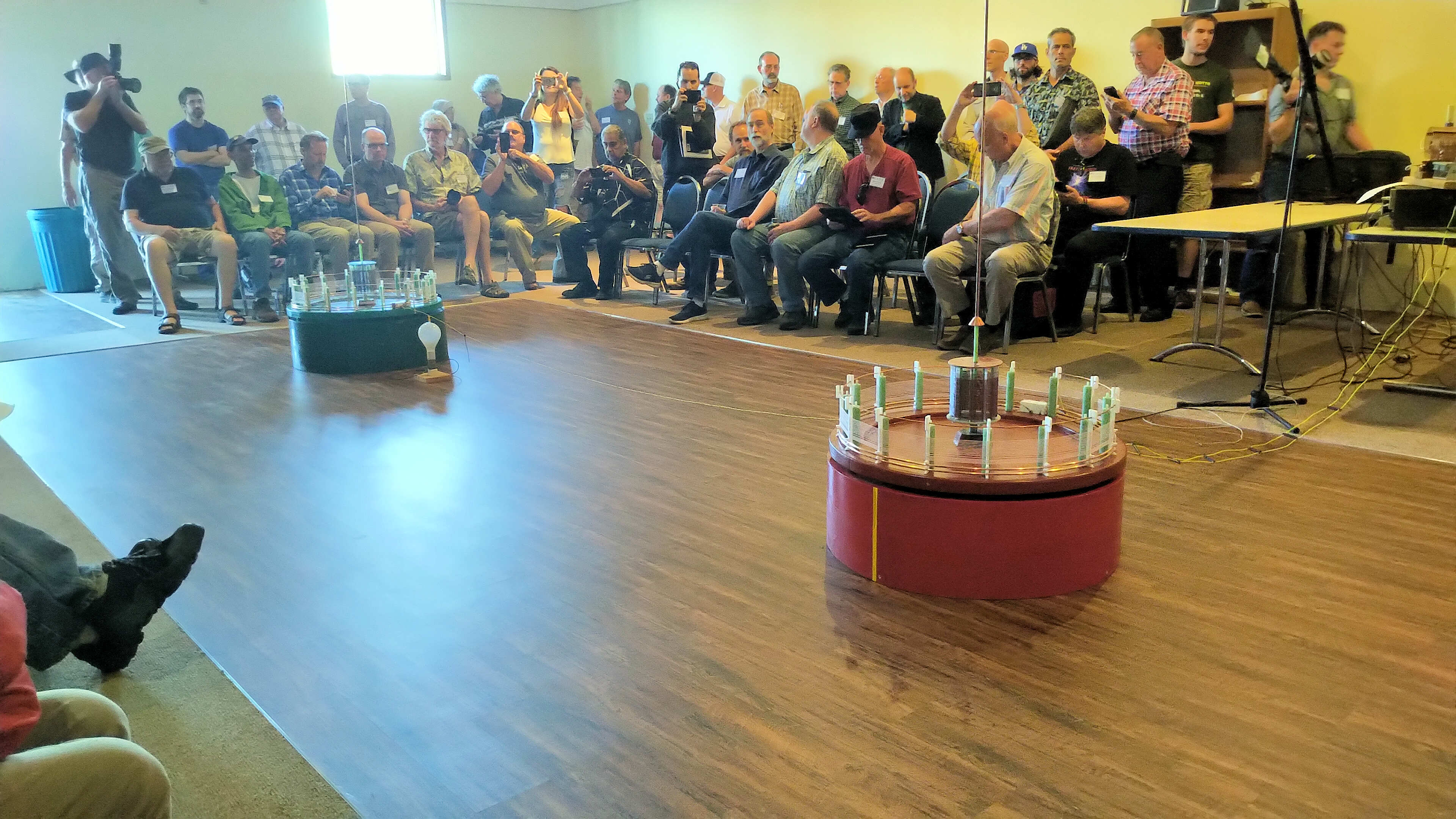
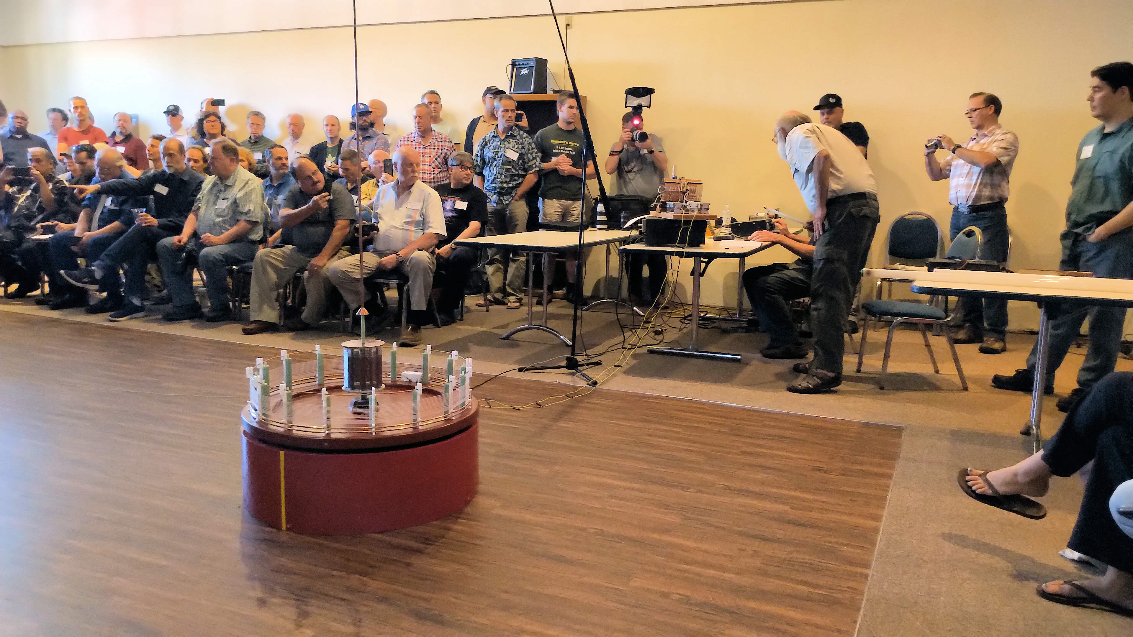
ESTC 2019, the Energy, Science, and Technology Conference^[1], included a presentation and working demonstration by Eric Dollard on Tesla’s Colorado Springs experiment^[2] (TCS), which is available through A & P Electronic Media^[3,4]. Due to unforseen circumstances relating to the demonstration co-worker, the generator for this experiment was unavailable after the demonstration for additional experimentation, investigation, and follow-up demonstrations. In agreement with Eric Dollard I suggested that the spark gap generator from the Vril Science Multiwave Oscillator Product^[5], (MWO), could be adapted, tuned, and applied to the Colorado Springs experiment, and in order to facilitate ongoing investigation and experimentation throughout the conference period. What follows in this post is the story of how this successful endeavour unfolded in the form of videos, pictures, measurements, and of course the final results.

The first video below shows highlights from the endeavour, video footage was recorded and supplied by Paul Fraser, and reproduced here with permission from A & P Electronic Media.

The second video below shows highlights from the impedance measurements part of the endeavour, video footage again by Paul Fraser, and by Raui Searle.

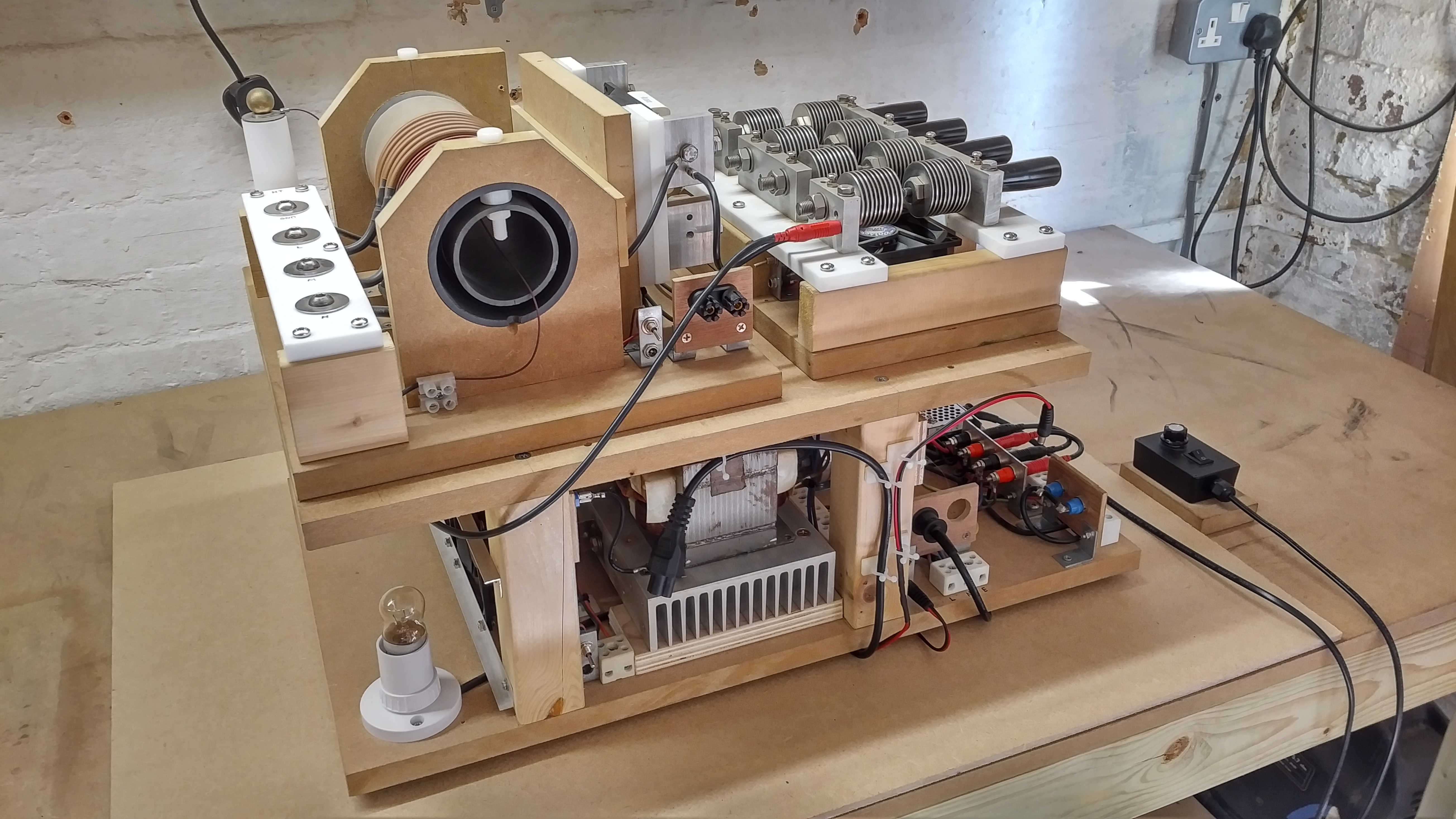
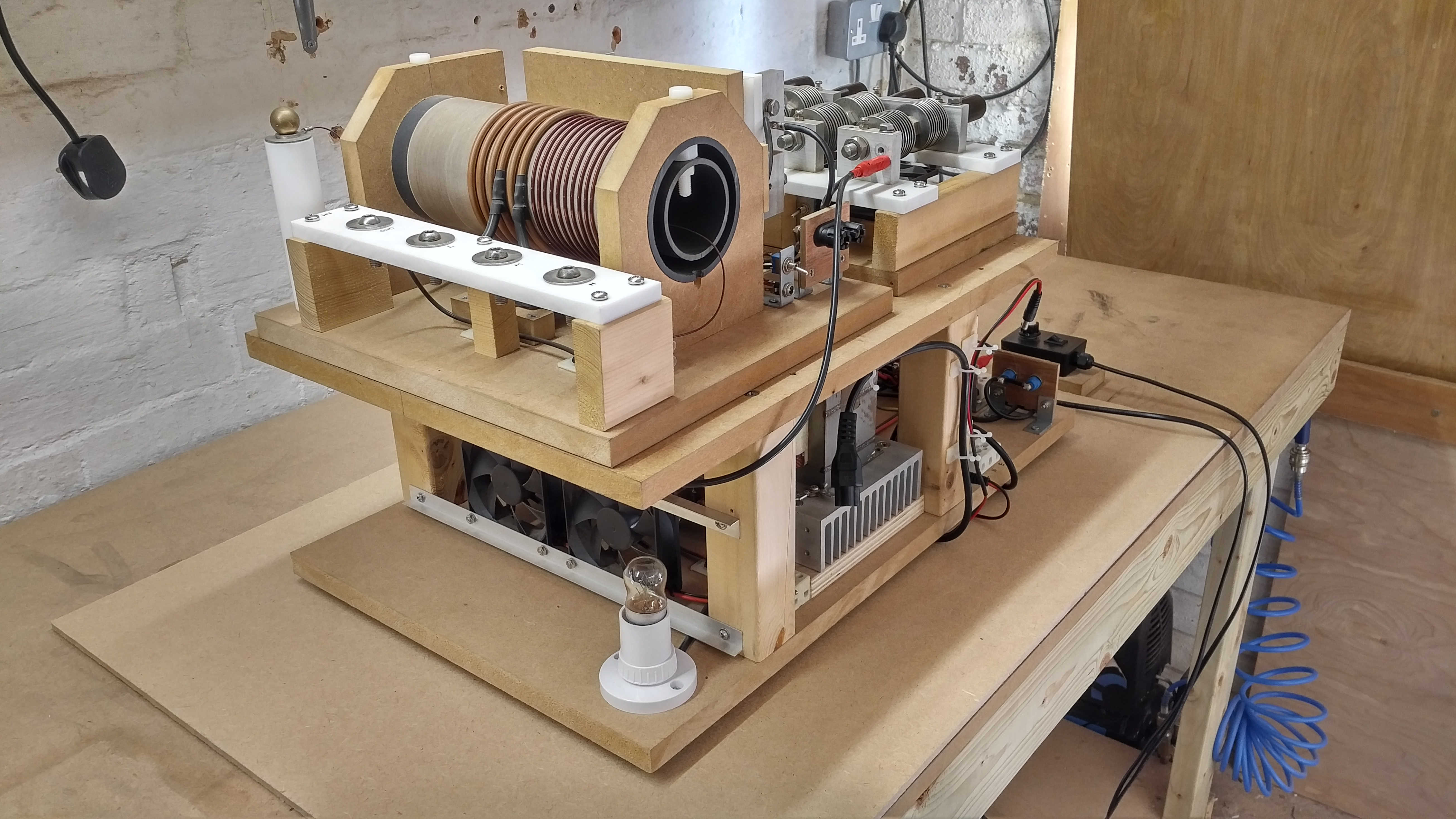
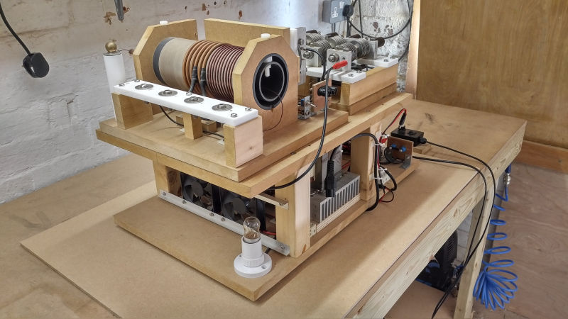
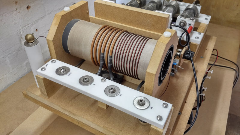
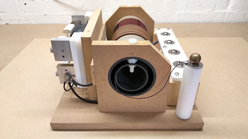
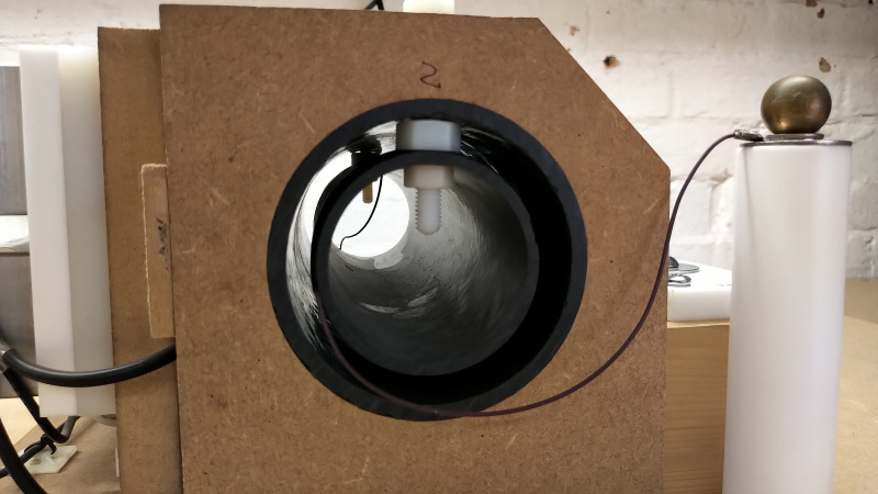
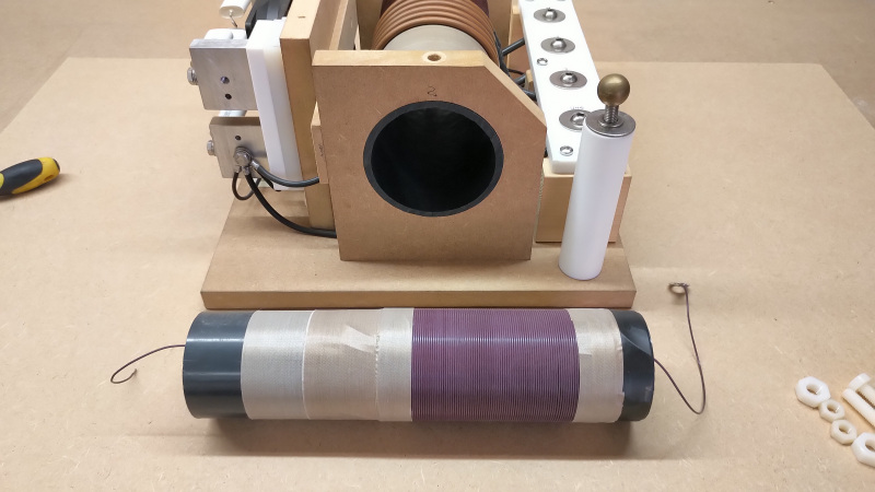
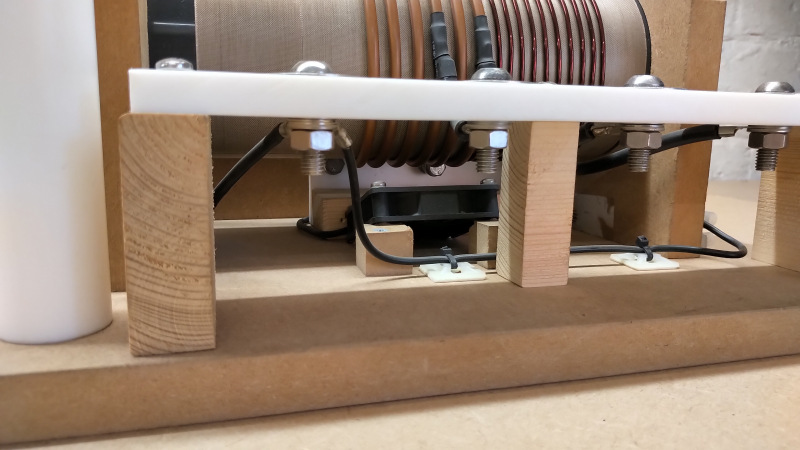
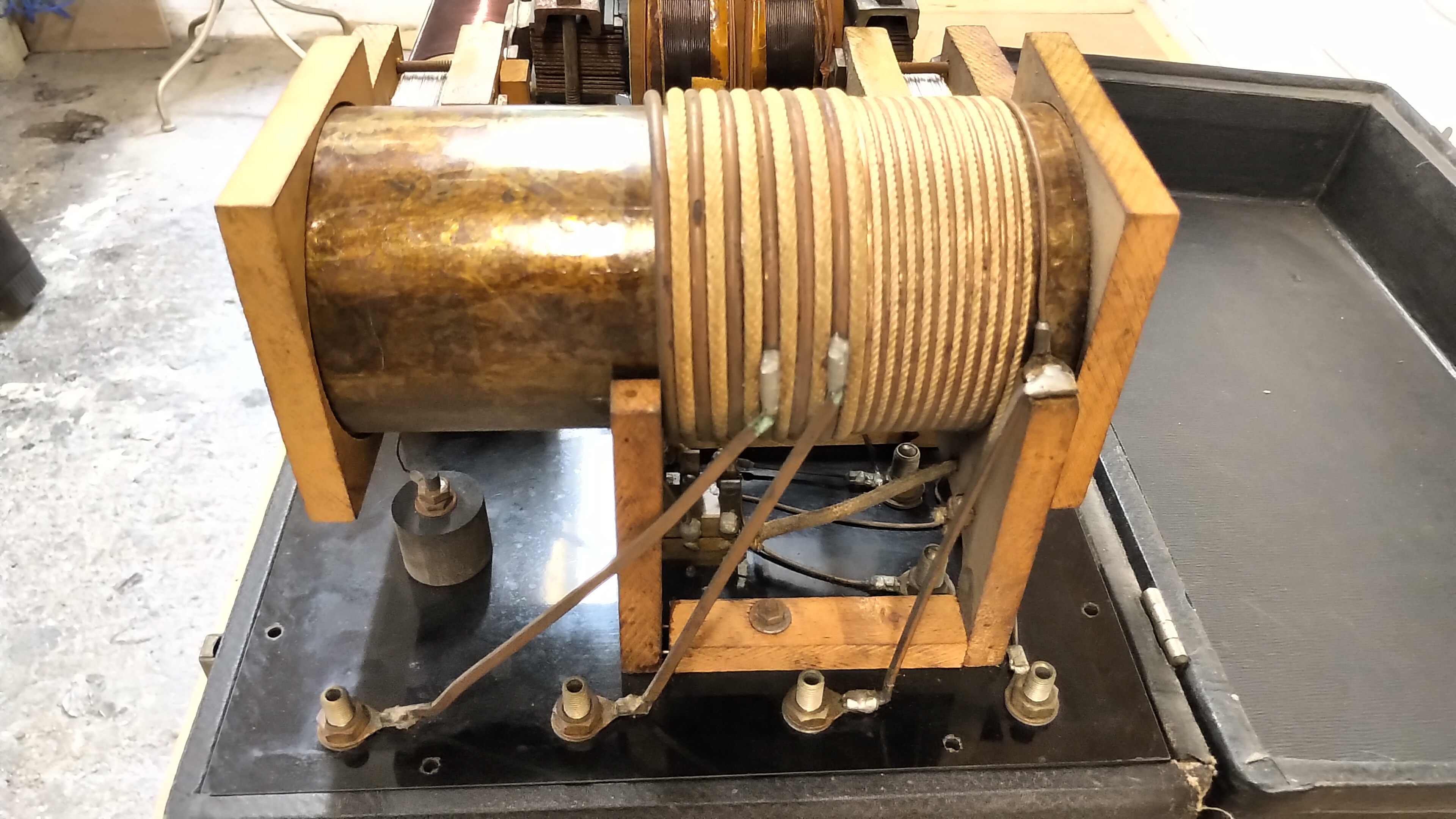
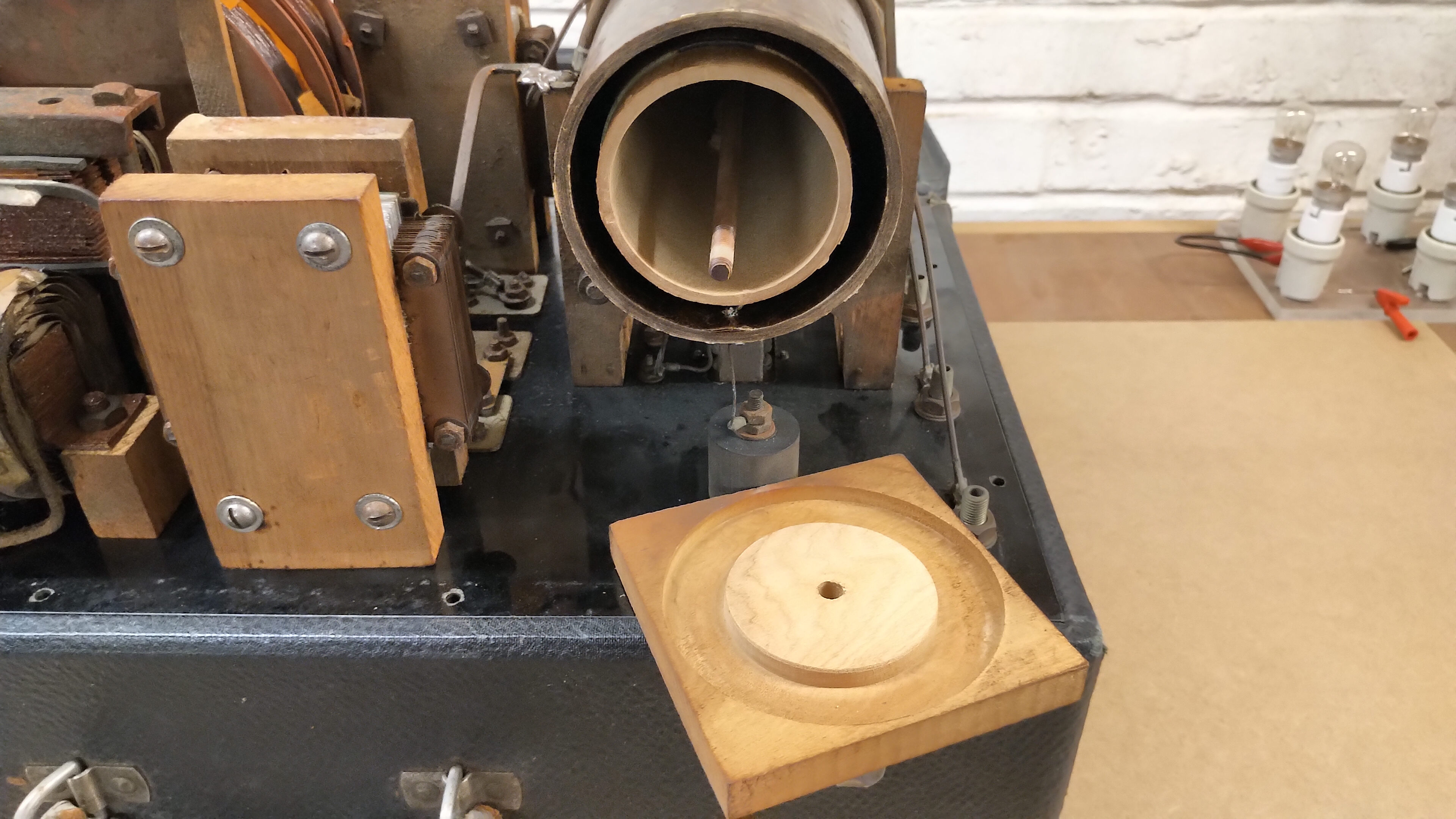
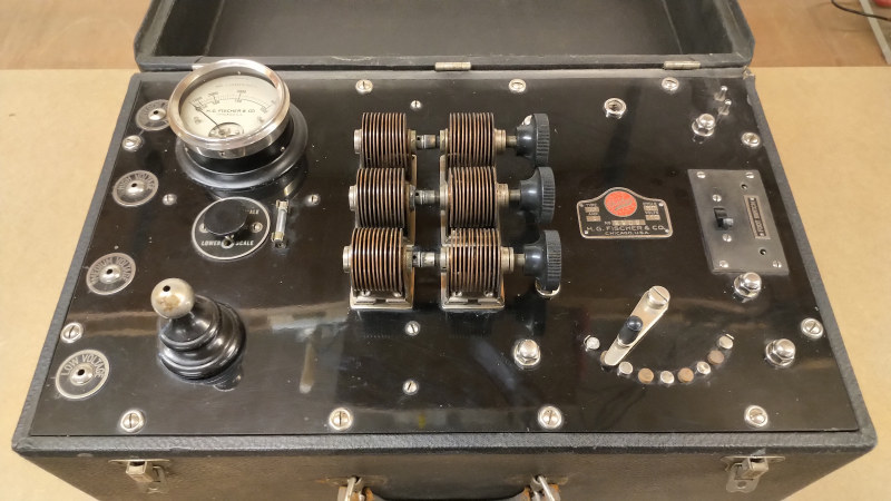
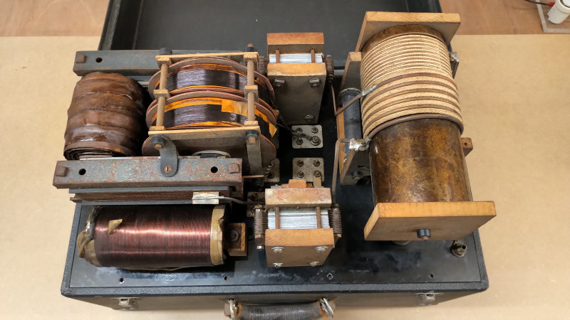
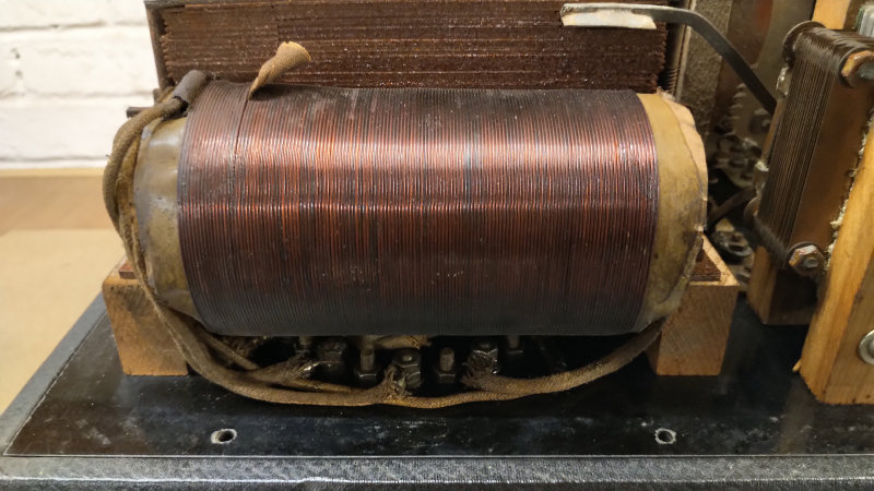
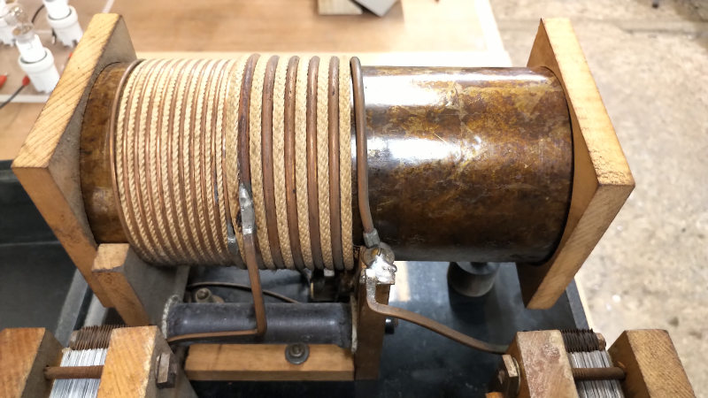
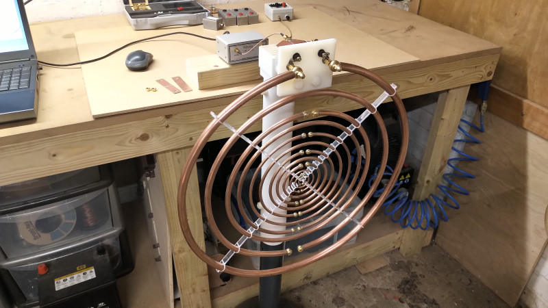
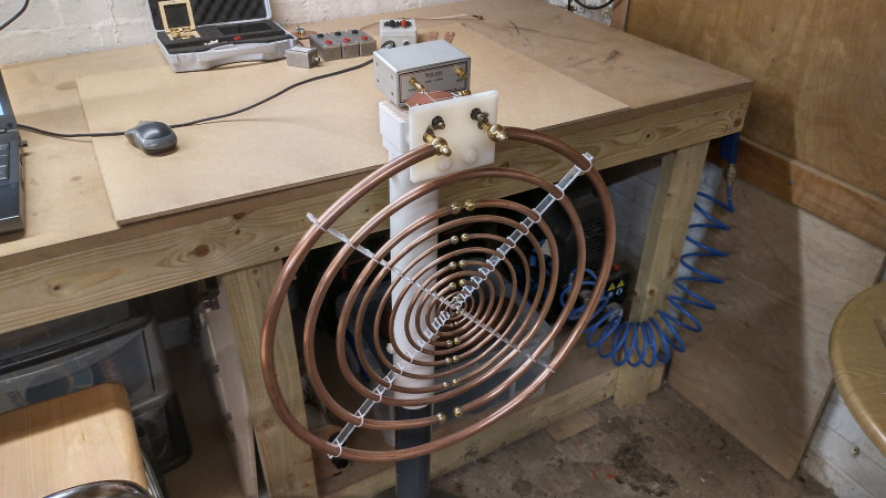
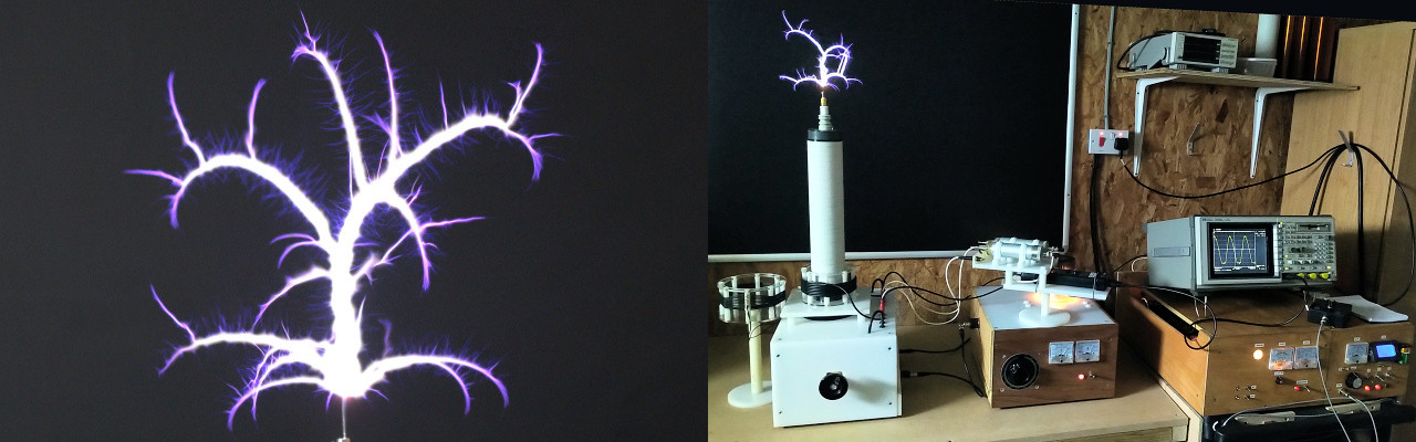
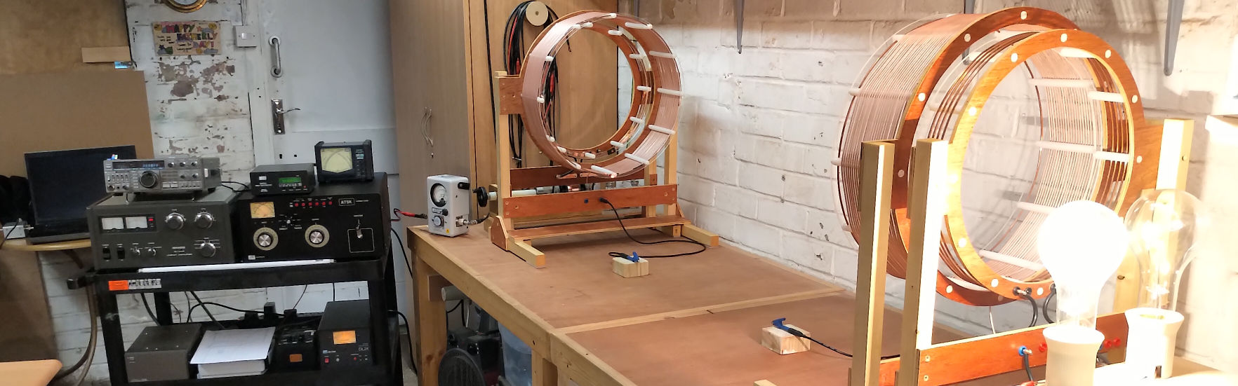
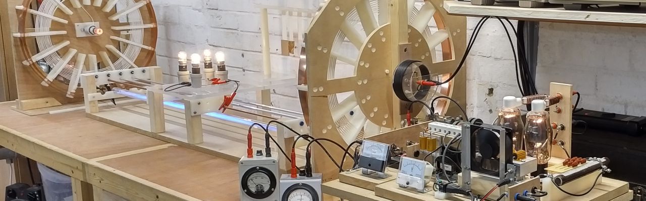
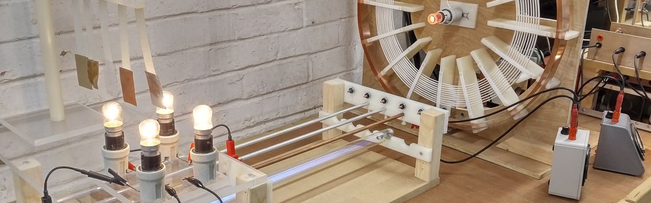
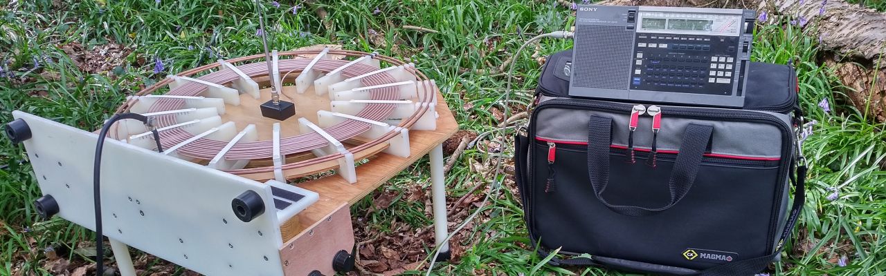
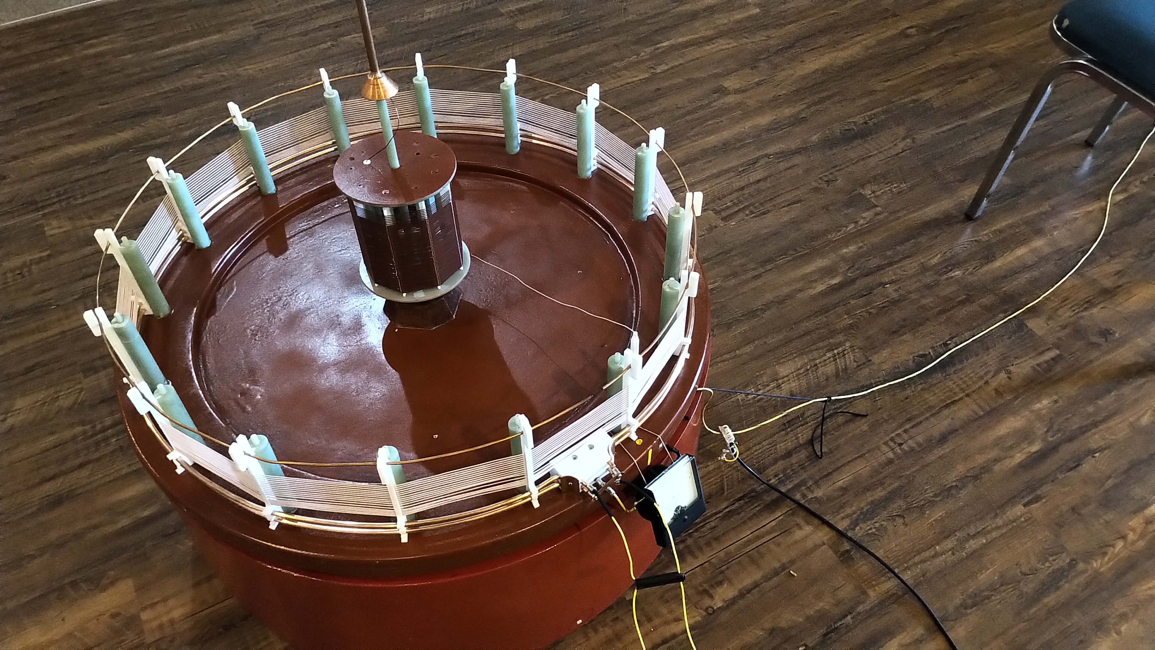
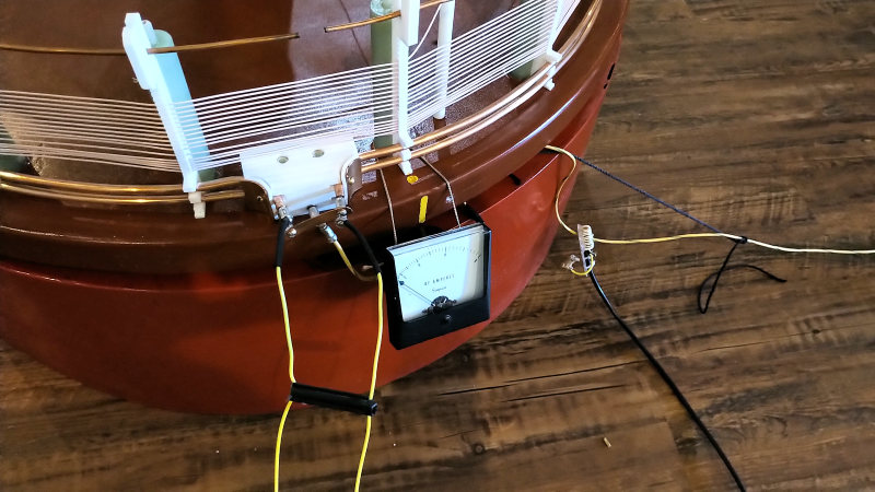
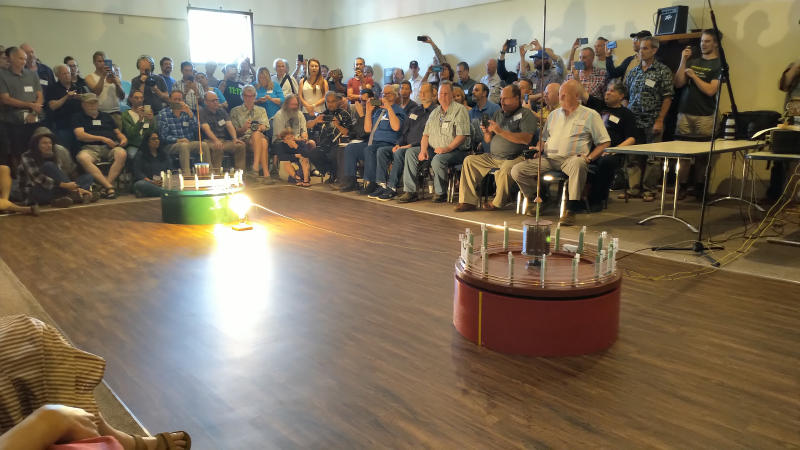
Figures 1 below show a range of pictures of the original transmitter and receiver setup from Eric Dollard’s TCS demonstration, including the generator used to power the experiment, and key results from the original demonstration. The red “transmitter” coil (RTC) was subsequently modified after the demonstration, (secondary coil re-wound, and with a single copper strap primary), in order to work well with the MWO spark gap generator. The green “receiver” coil (GRC) was left un-modified for the purpose of the endeavour, although it could be fine tuned using the extra coil telescopic extension. Ultimately for on-going experiments using the MWO generator, the GRC would be re-wound and adapted to more closely match the RTC.

Fig. 1.1 The coil arrangement for the TCS demonstration by Eric Dollard, showing both the red transmitter coil and the green receiver coil.
Fig. 1.2 The red transmitter coil showing the general arrangement of the primary, secondary, and the extra coil.
Fig. 1.3 The generator is connected to the primary via a balanced transmission line, and the secondary is connected to the green receiver coil via an rf ammeter.
Fig. 1.4 The receiver load is a 500W incandescent light bulb, connected to the primary of the receiver coil. The receiver is connected by a single wire to the transmitter.
Fig. 1.5 The linear amplifier is a 1000W Denton Clipperton-L, and is connnected to the red transmitter coil via a matching unit.
Fig. 1.6 The linear amplifier output matching unit is in itself a tuned resonant transformer, which matches the output of the amplifier on the 160m band to the much lower impedance of the primary in the MW band.
Fig. 1.7 The output of the matching unit is via variable high voltage tuning capacitors in parallel with the output coil.
Fig. 1.8 The input to the matching unit is via a balanced transmission line to a tuned vacuum capacitor, and in parallel with the twin series connected input coils.
Fig. 1.9 The signal source for the linear amplifier is from an ICOM 7300 amateur radio receiver, modified to transmit on the MW band at 848.4kc/s.
Fig. 1.10 The Denton linear amplifier has no matching input network, hence a matching unit is required between the ICOM 7300 transceiver and the amplifier.
Fig. 1.11 All parts of the system connected together prior to the beginning of the demonstration.
Fig. 1.12 Last minute tuning checks by Eric Dollard prior to turning up the power for music transmission to the green receiver via the MW band.
Fig. 1.13 Checking for a null point between the transmitter and the receiver using a domestic flourescent tube to indicate the local electric field strength.
Fig. 1.14 Investigating the field around the extra coil extension using a helium-neon tube.
Fig. 1.15 Transmission of electric power from the transmitter to the receiver via a single wire, and lighting fully a 500W incandescent bulb.

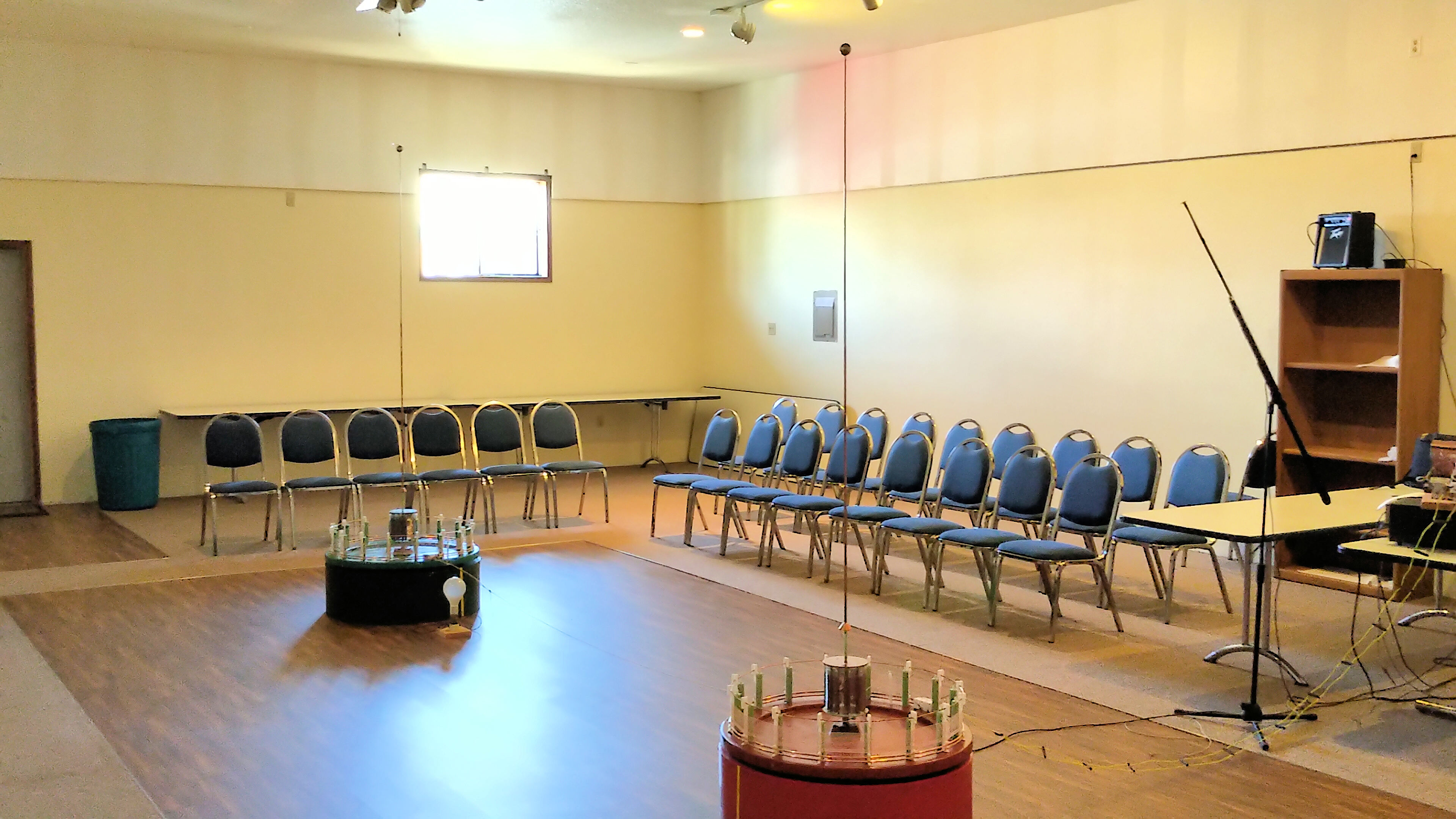
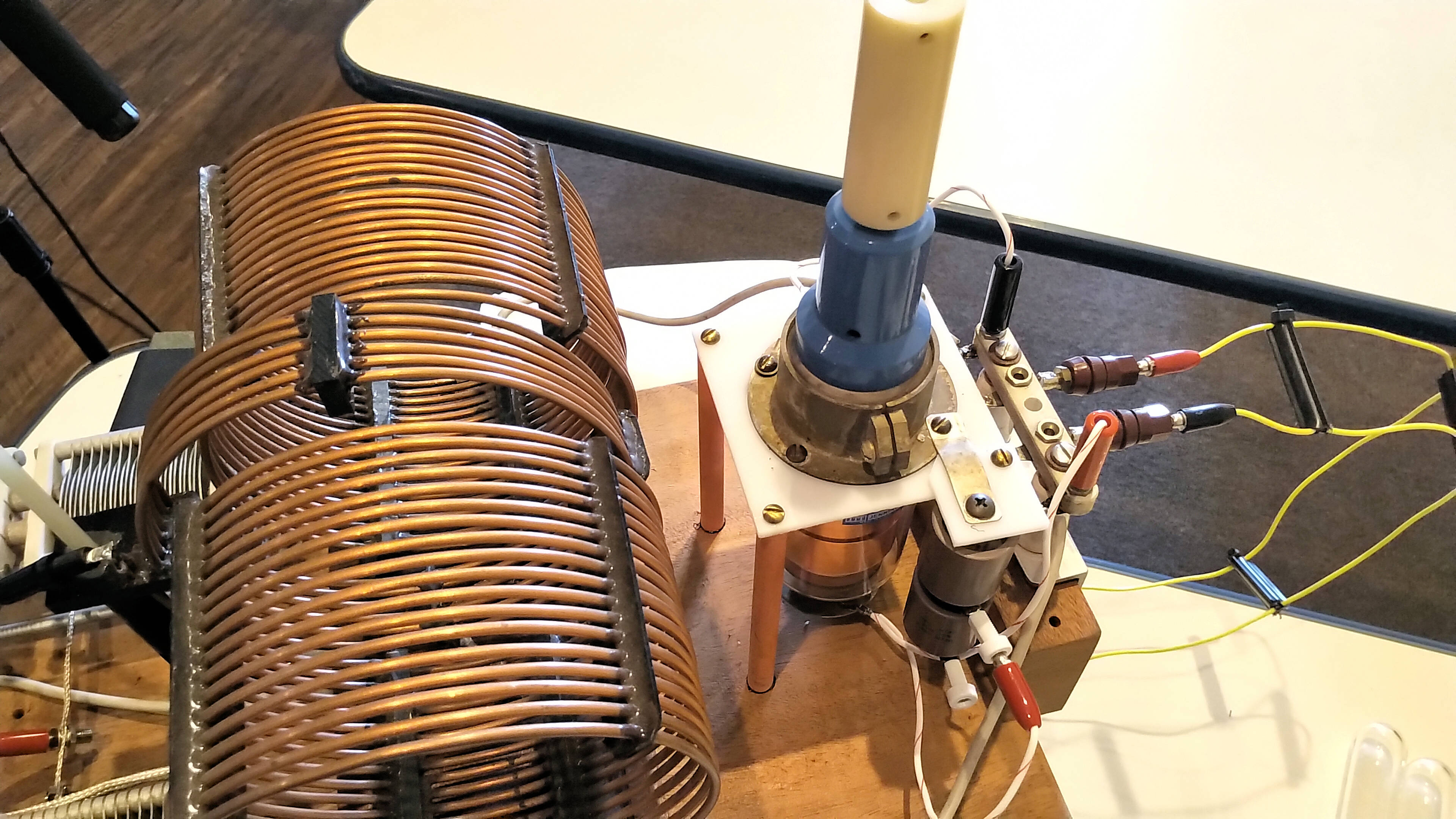
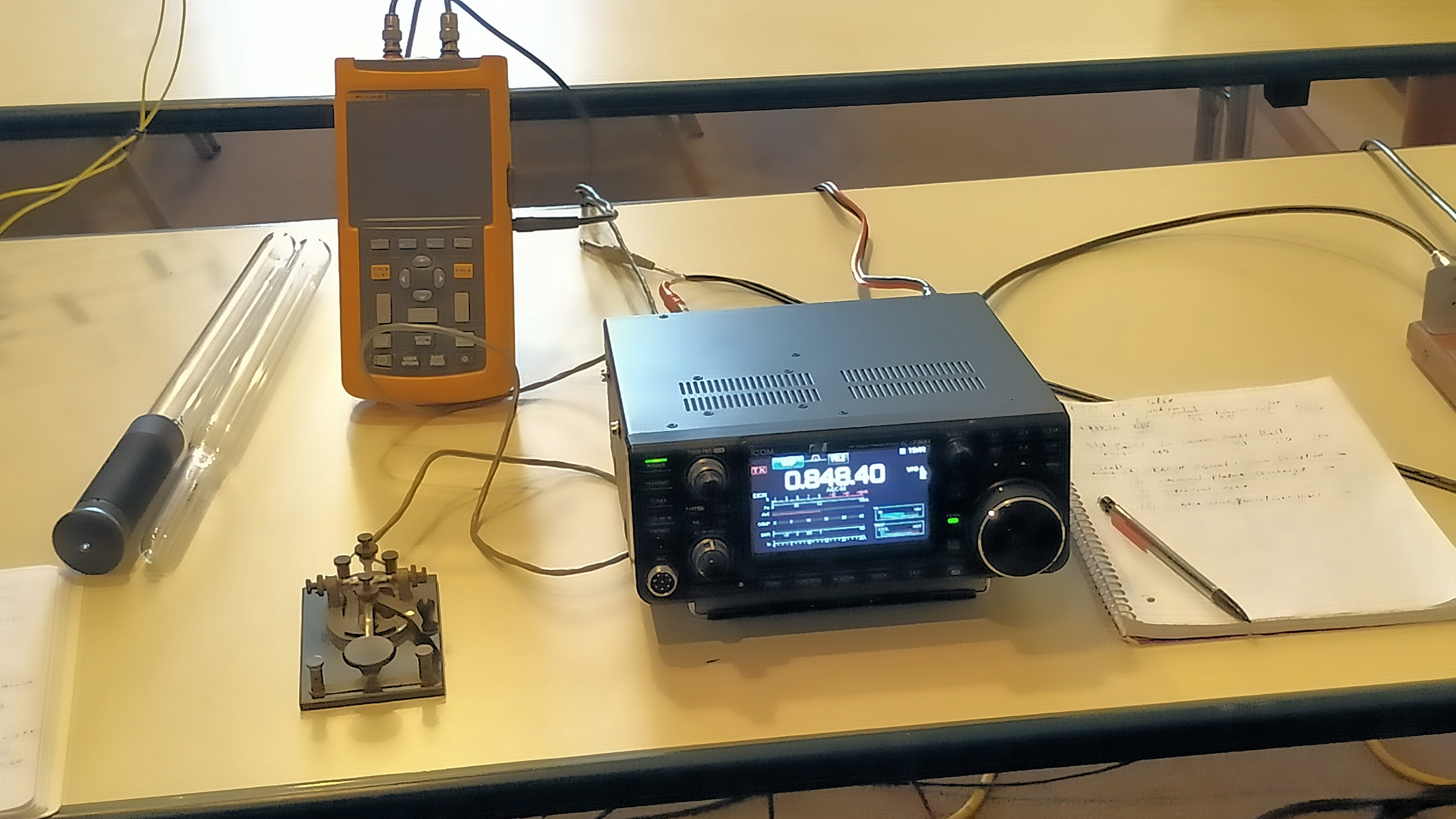
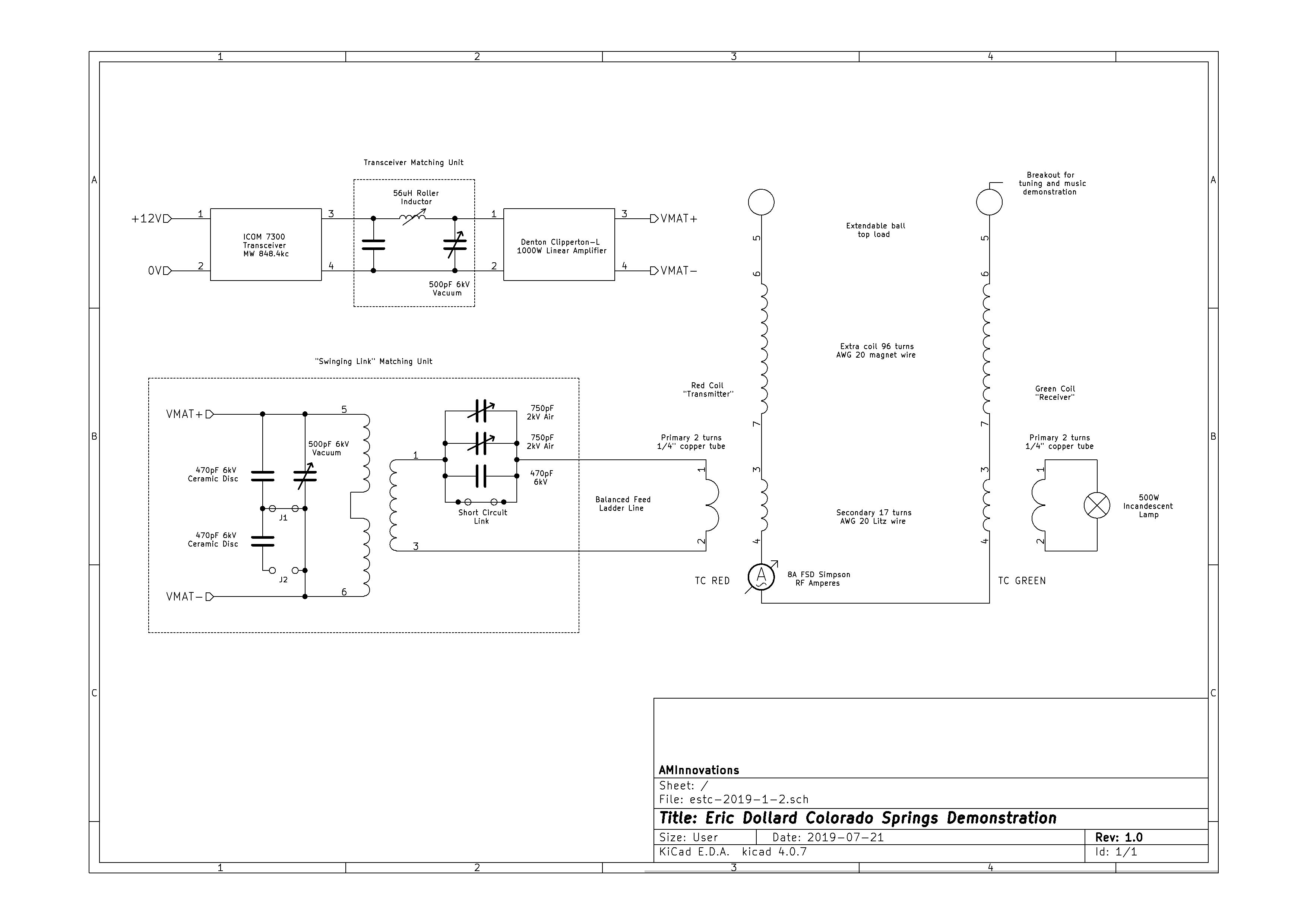
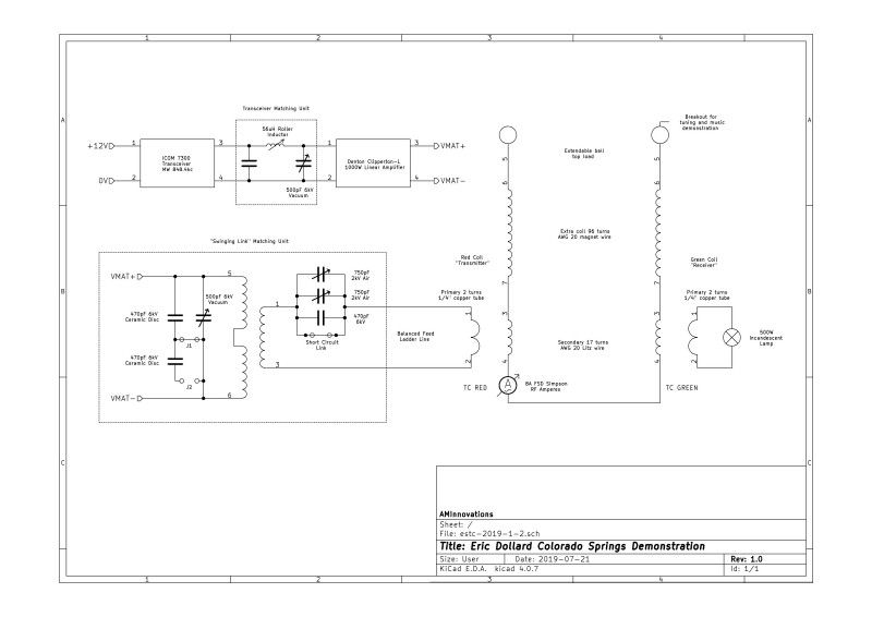
The original TCS demonstration was powered by a 1000W linear amplifier generator being driven at ~ 800W output to light a 500W incandescent bulb at the receiver primary, and where the electric power is transferred between the RTC and GRC by a single wire. The TCS demonstration with both coils fully configured and connected to the generator was tuned to a drive frequency of 848.4 kc/s, as can be seen in fig. 1.9 as the selected frequency of the transceiver.

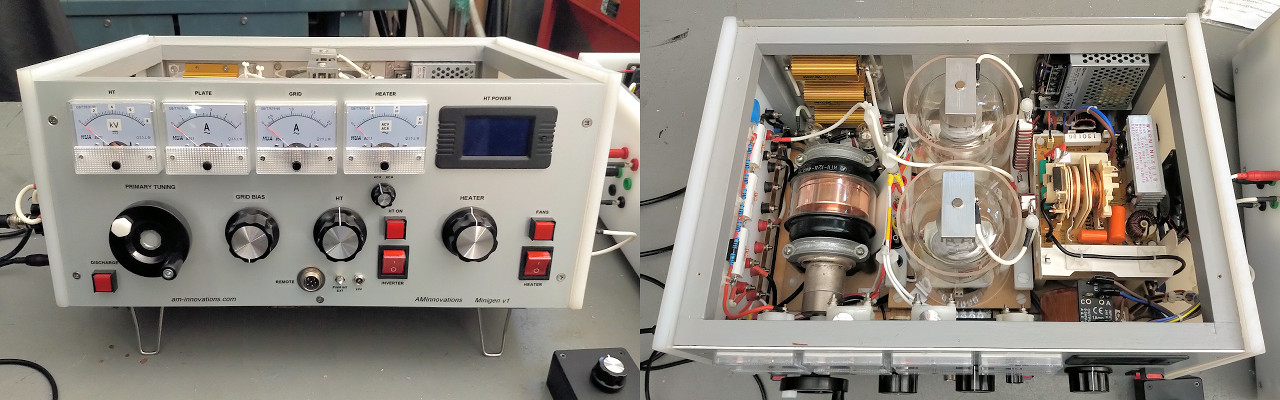
The transceiver is an ICOM-7300 which must have been modified to allow transmit on all frequencies, a modification that allows a radio amateur transceiver to generate a transmit signal outside of the designated amateur bands. This kind of modification turns a transceiver into a powerful bench top signal generator, with full modulation capabilities, and matched output powers from the transceiver alone of up to 100W in the MF and HF bands (300kc/s – 30Mc/s). 848 kc/s is in the MW (MF) radio broadcast band, and amplitude modulation is well suited here for the transmission of voice and music signals, as was also demonstrated in the original experiment.

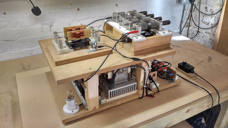
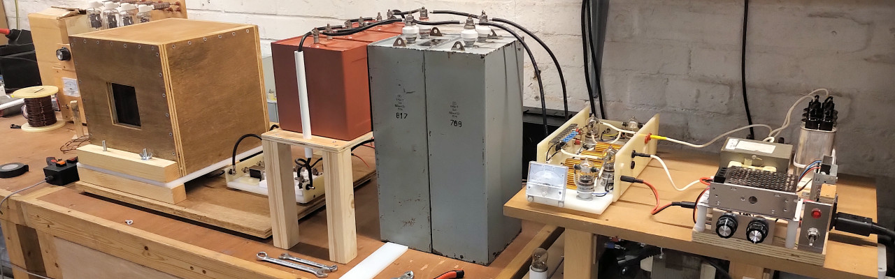
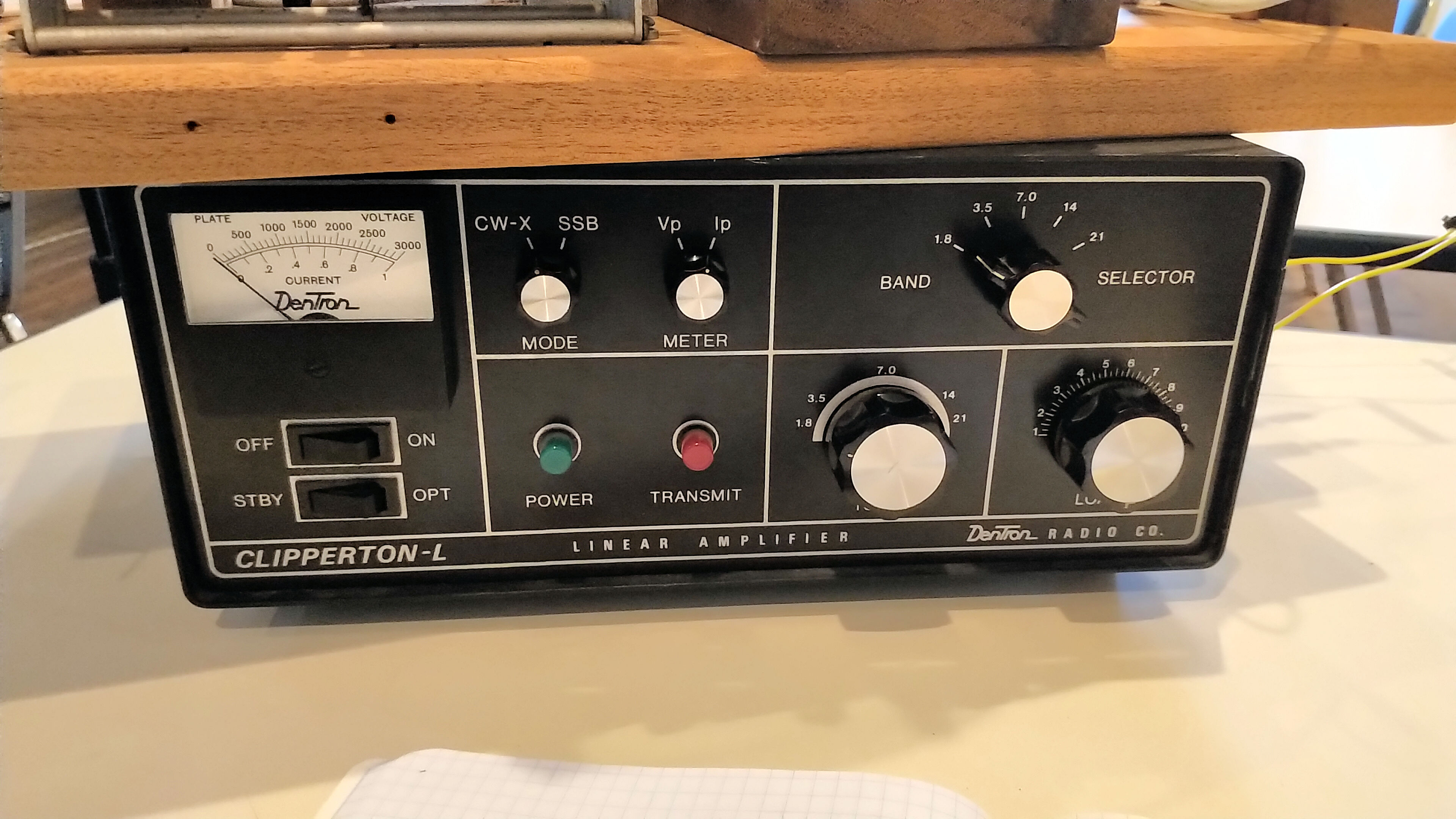
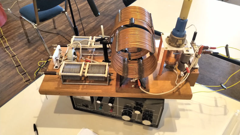
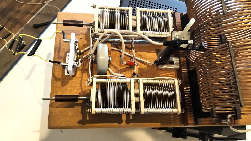
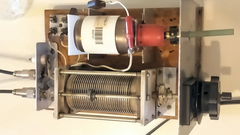
The ICOM transceiver is connected via a matching unit to the Denton linear amplifier. This specific brand and model of linear amplifier has no matching unit at its input, which is why external matching is required from the ICOM 50Ω output to the lower impedance Denton input. The passive matching unit is shown in fig. 1.10, and also in the schematic of fig. 2.1.

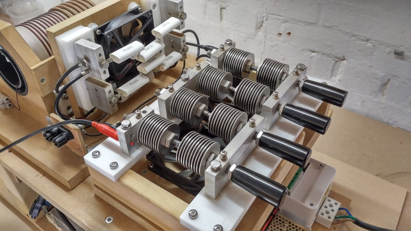
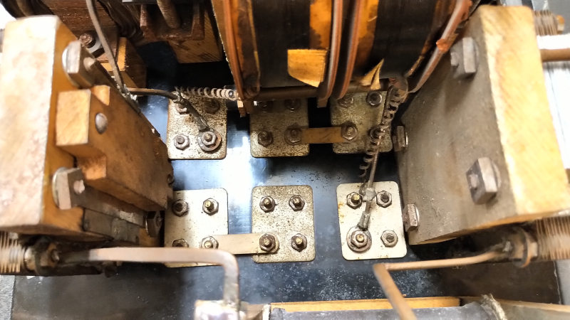
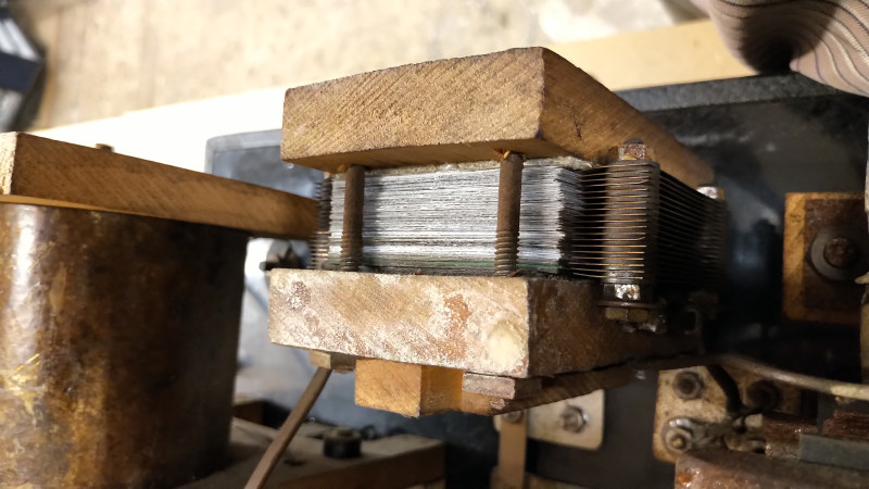
The Denton Clipperton-L is a linear amplifier using 4 x 572B vacuum tubes with a band selected matching unit at its output, and a total output peak voltage of ~ 500V. The lowest band provided internally for matching at the output of the amplifier is the HF 160m band at ~ 1.8Mc/s. The much lower MW signal at 848kc/s would need additional matching and balancing between the amplifier output and the input to the primary of the RTC, (the output of the amplifier is an unbalanced feed e.g. coaxial, whereas the connecting transmission line and the primary are better fed with a balanced feed). The amplifier passive matching unit is shown in figures 1.6 – 1.8, and is also shown in the schematic of fig. 2.1.

The various different experiments conducted in the original demonstration included the following:

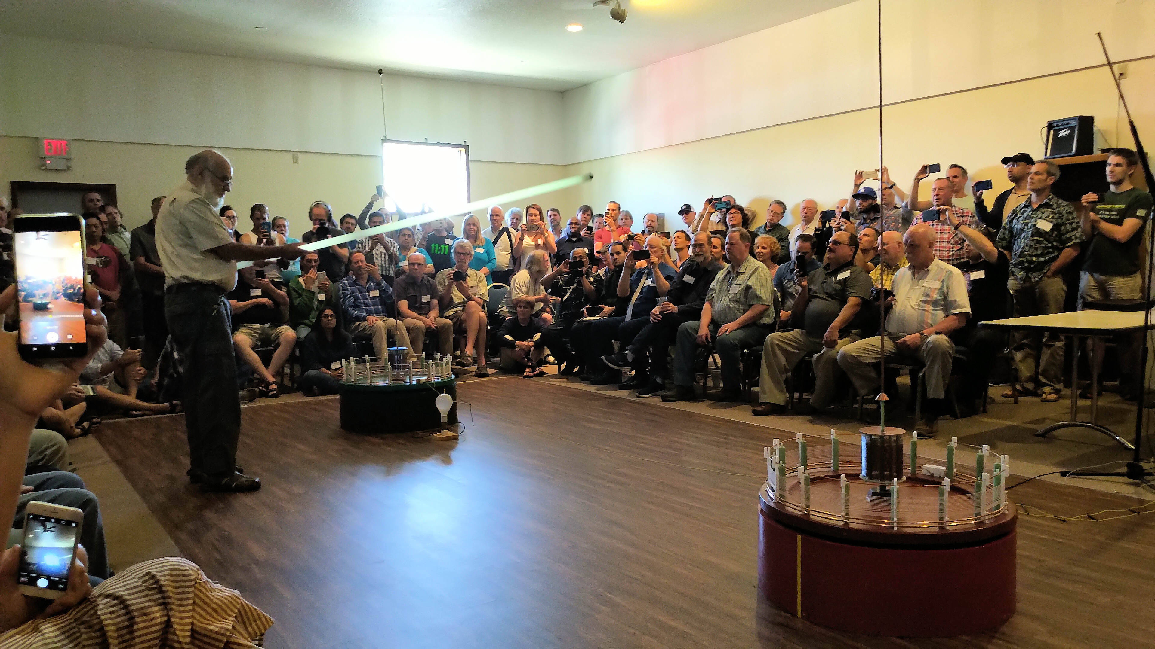
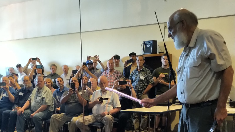
Fig 1.13. Shows Eric Dollard finding the null electric field region between the RTC and GRC, and using a 6′ domestic fluorescent tube light.

Fig 1.14. Shows Eric Dollard testing the field surrounding the RTC extra coil extension top load, using a helium-neon gas filled tube.

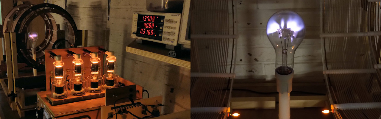
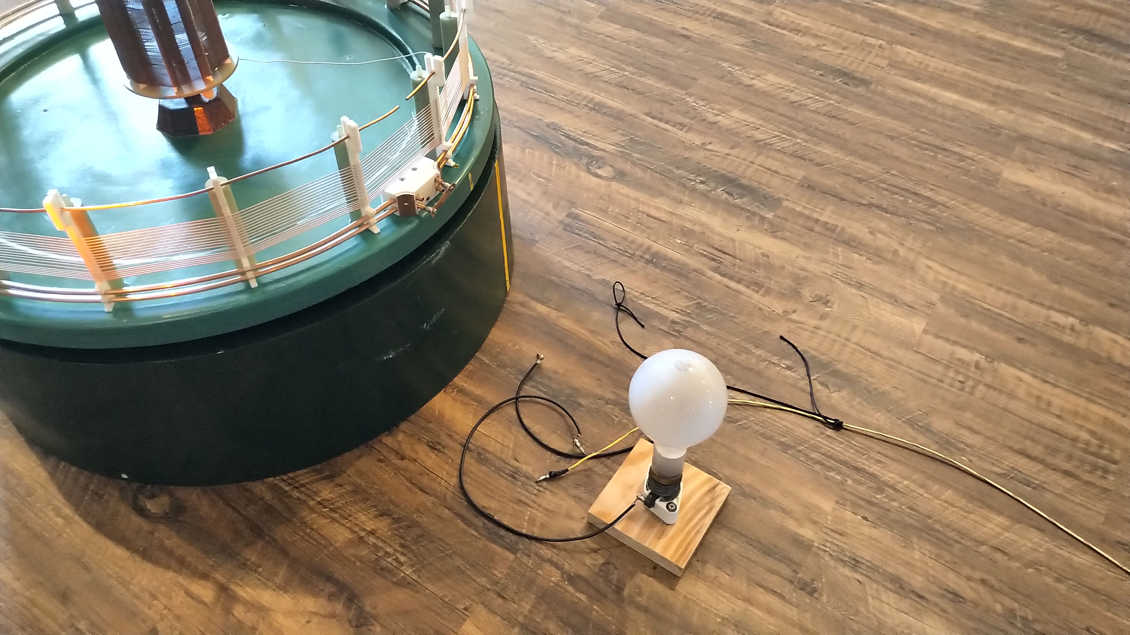
Fig 1.15. Shows single wire transmission of electric power, and fully lighting a 500W incandescent light bulb at the primary of the GRC.

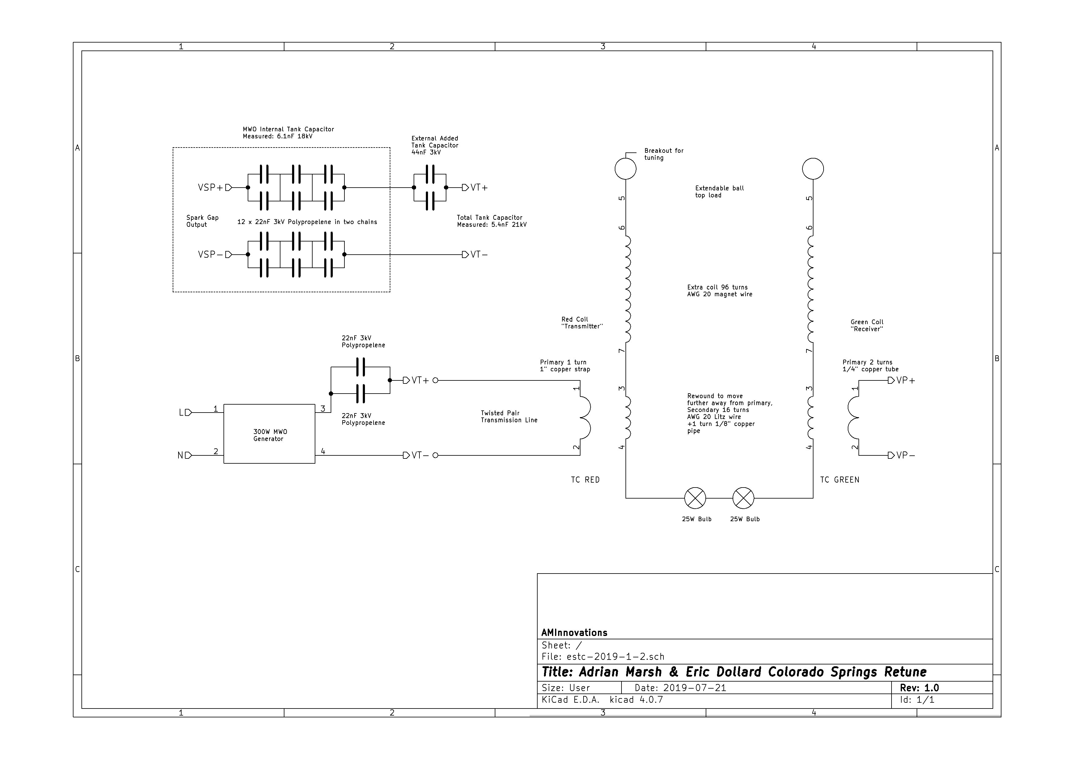
Figures 2 below show the schematics for both the linear amplifier generator and coil arrangement for Eric Dollard’s original TCS demonstration, and a second schematic for the TCS experiment retune using the MWO spark gap generator. The high-resolution versions can be viewed by clicking on the following links TCS Demonstration, and TCS Retune.

Fig. 2.1 Schematic diagram for the TCS demonstration by Eric Dollard, showing the generator, matching units, and coil arrangements.
Fig. 2.2 Schematic diagram for the TCS retune by Adrian Marsh & Eric Dollard, showing the MWO generator, tuning capacitors, and modified coil arrangements.

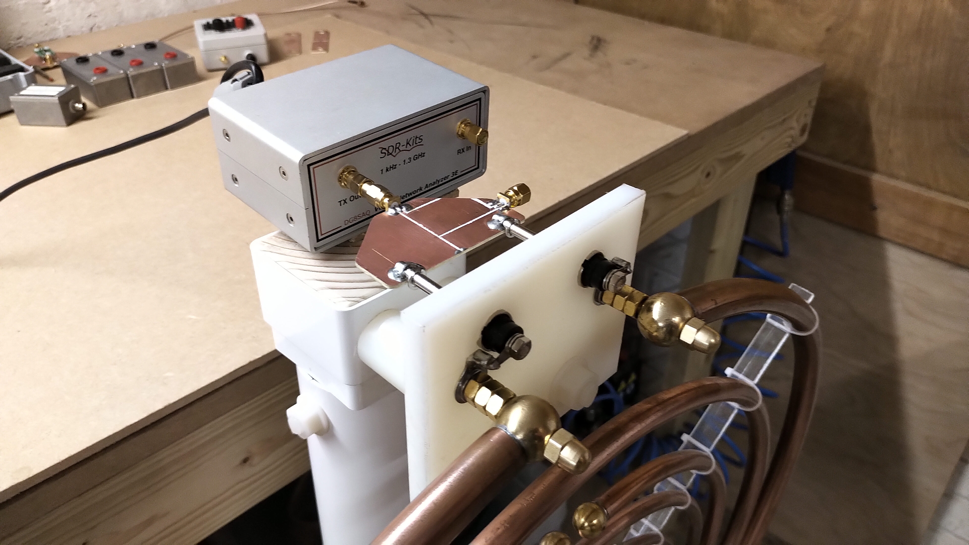
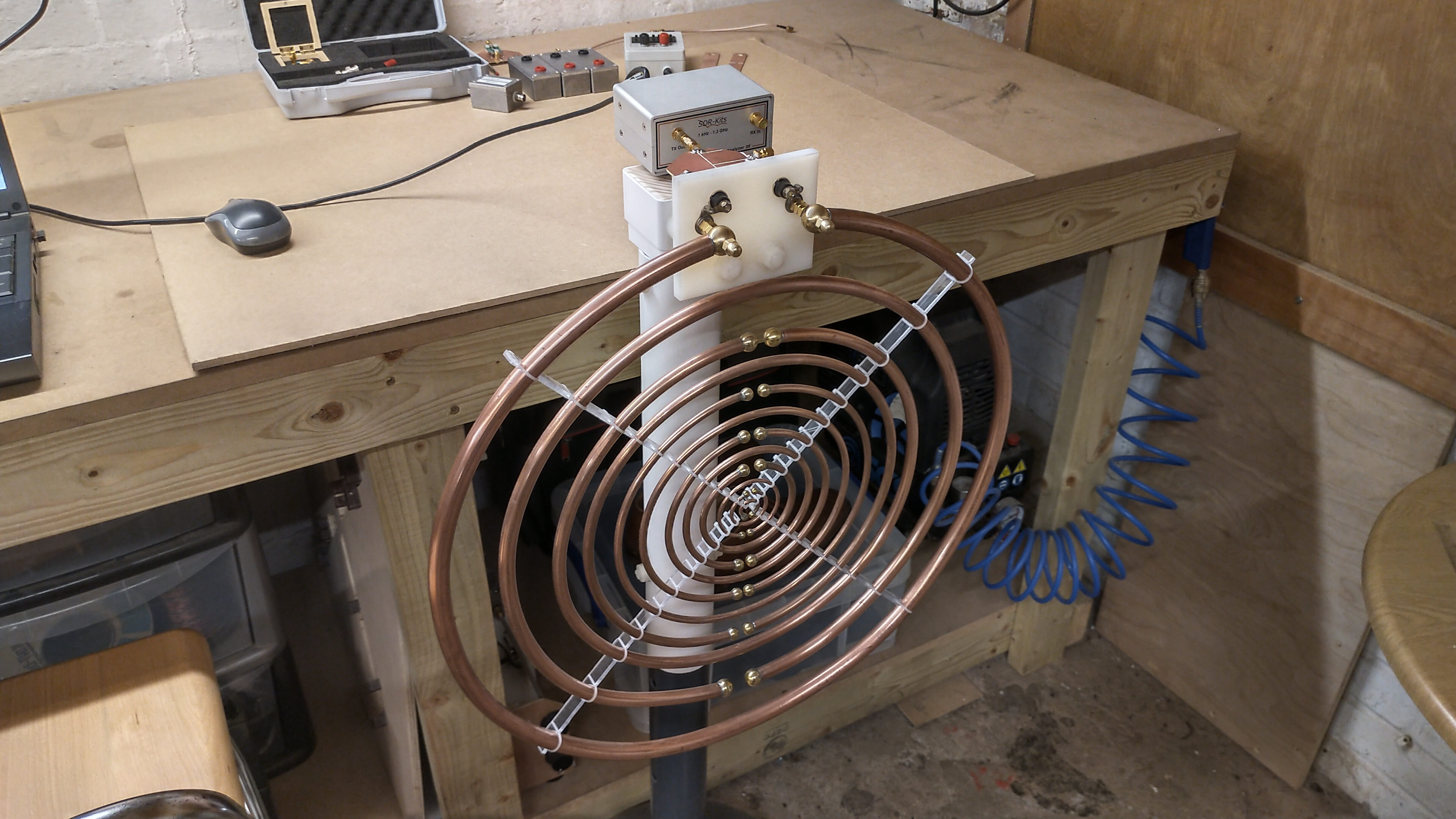
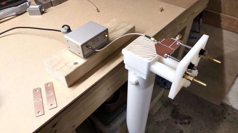
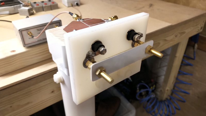
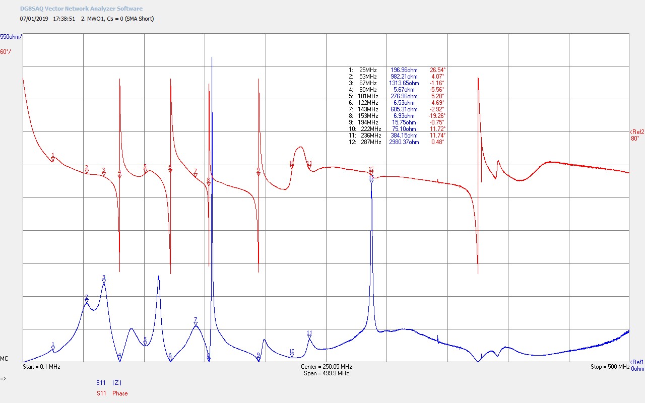
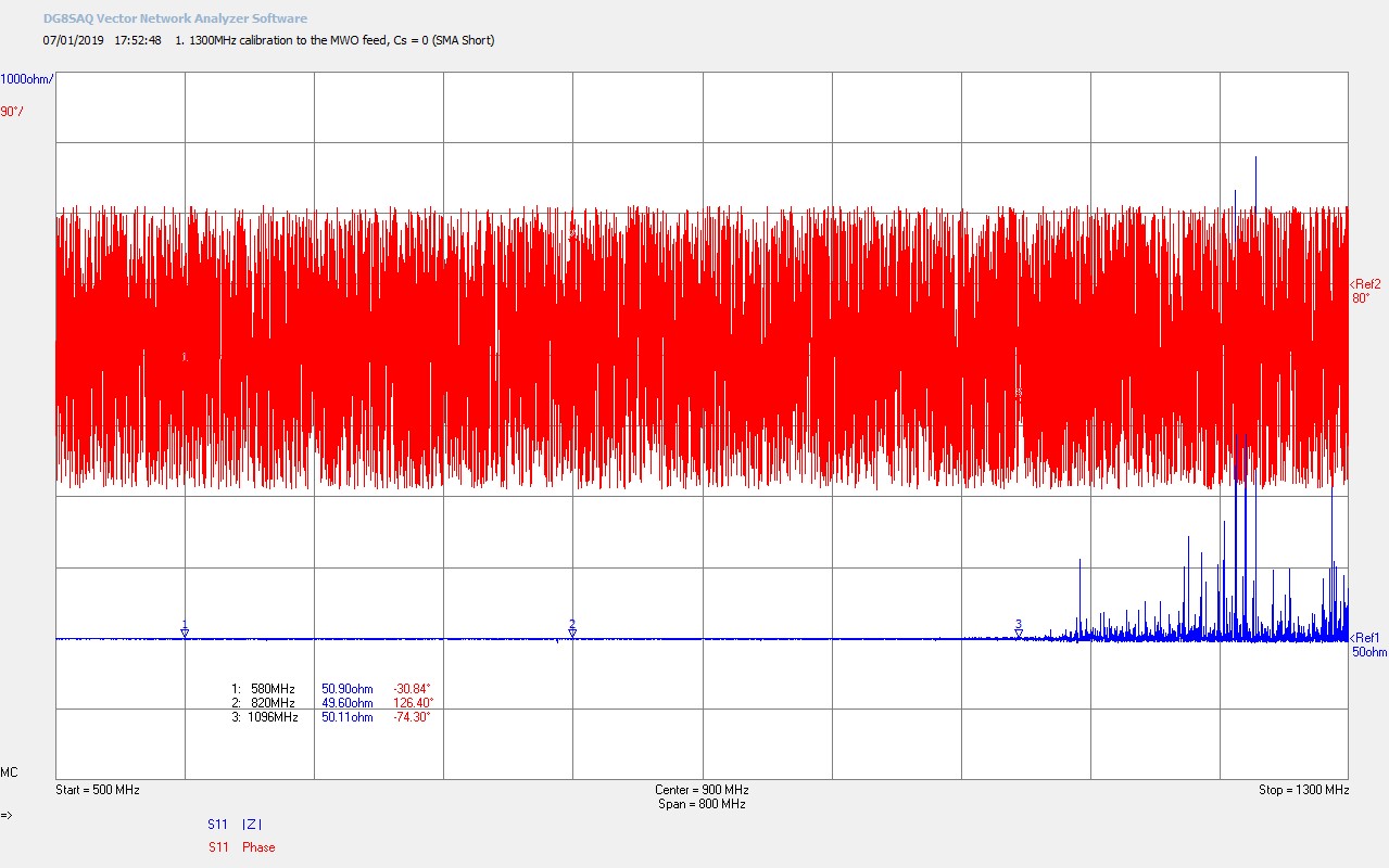
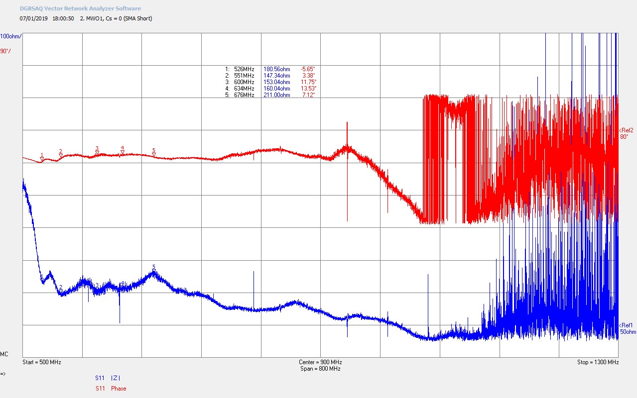
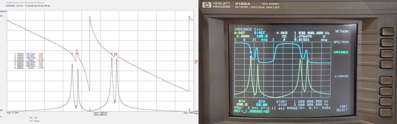
Figures 3 below show the small signal impedance measurements for Z₁₁ for the TCS coils, and also the tuning measurements for the coils and spark gap generator together, which were taken throughout the endeavour and used to ensure a well tuned match between the generator and the TCS experiment.

Fig. 3.1 Shows the Z11 impedance for the RTC with the extra coil not connected. The bottom end of the secondary is grounded.
Fig. 3.2 Shows the secondary and the extra coil connected together. The bottom end of the secondary is grounded, and the extra coil extension aerial is fully extended.
Fig. 3.3 The RTC and GRC are connected by a single wire, and with both extra coil aerial extensions fully extended.
Fig. 3.4 The RTC and GRC are connected by a single wire, and with both extra coil aerial extensions adjusted to balance the impedance of the fundamental resonant frequency.
Fig. 3.5 The RTC consisting of a 2 turn copper pipe primary, secondary, and extra coil with extension is connected to the MWO generator at the spark gap outputs, showing the overall tuning from the perspective of the generator.
Fig. 3.6 The RTC consisting of a 1 turn copper pipe primary and connected to the MWO generator at the spark gap outputs.
Fig. 3.7 The RTC with a 1 turn copper strap primary connected to the output tuned MWO generator at the spark gap outputs, and showing a clean tuning for the fundamental resonant frequency at 822kc/s.

To view the large images in a new window whilst reading the explanations click on the figure numbers below, and for a more detailed explanation of the mathematical symbols used in the analysis of the results click here. For further detail in the analysis and consideration of Z₁₁ typical for a Tesla coil based system click here.

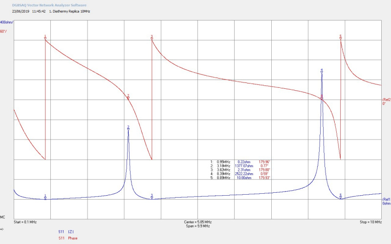
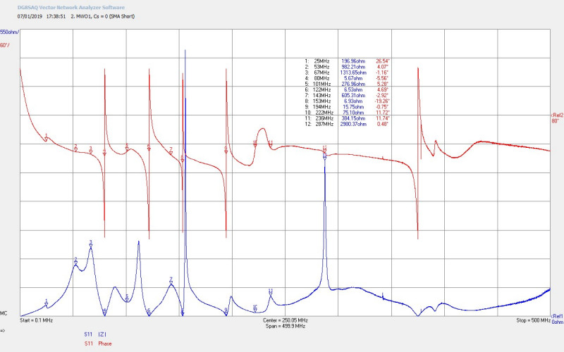
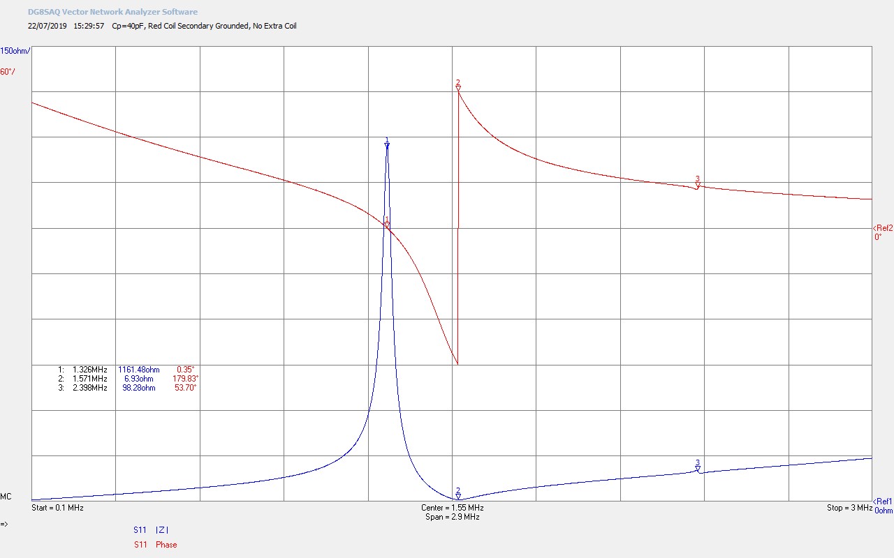
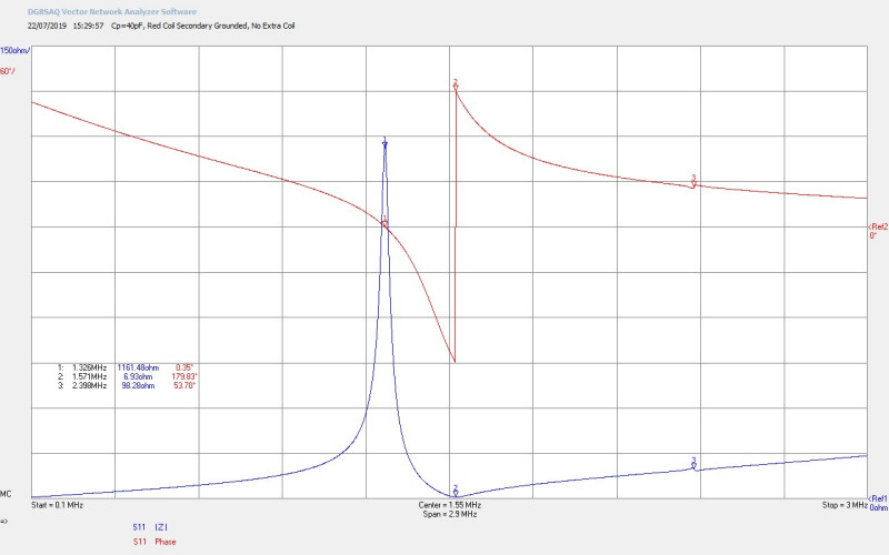
Fig 3.1. Shows the impedance measurements for the RTC with the secondary grounded, the extra coil disconnected, and where the primary tank capacitance has been arranged to be series C_P= 40pf, which puts the primary resonant frequency F_P at a much higher frequency and far away from the secondary. This would be the proper drive condition for the original linear amplifier generator (LAG) where F_P is not arranged to be equal to F_S. For the spark gap generator (SGG) it is necessary to match F_P as closely as possible to the combined resonant frequency of the secondary and the extra coil together. The fundamental parallel resonant frequency of the secondary Fs at M₁ = 1326kc/s, and as is to be expected with this form of air-cored coil, the F_Ø180 or series resonant point at which a 180° phase change occurs, is at a higher frequency at 1571kc/s at M₂. At M₃ = 2398kc/s a tiny resonance is being coupled from the disconnected extra coil which, being mounted in the centre on axis with the secondary, is close enough to have a non-zero coupling coefficient, and hence show some slight resonation reflected into the measurement.

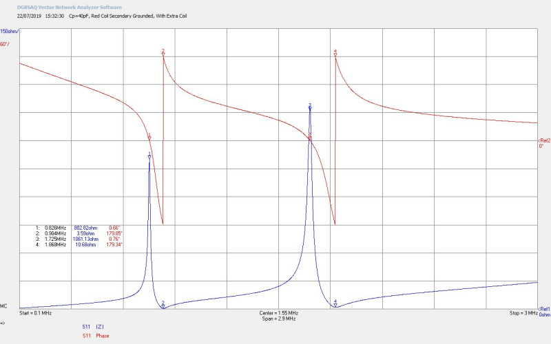
Fig 3.2. Here the extra coil has been reconnected and two resonant features can be noted, the lower from the secondary, and the upper from the extra coil. The effect of the coupled resonance between the two coils with a non-zero coupling coefficient is to push the secondary resonance down in frequency to where the F_S at M₁ is now at 826kc/s which is very close to the original drive frequency of the linear amplifier generator at 848kc/s. The fundamental resonant frequency of the extra coil, (now in λ/4 mode with one end at a lower impedance connected to the secondary, and the other connected to the high impedance of the extendable aerial), at M₃ is now 1725kc/s

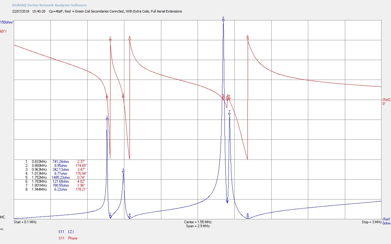
Fig 3.3. Here both the RTC and GRC have been connected together to complete the overall system, and where the bottom end of both secondaries are connected together by a single wire transmission line. Both the RTC and GRC have their extra coil adjustable extensions fully extended. It can be seen that both the secondary and extra coil resonant frequencies have been split in two, to reveal four resonant frequencies from the four main coils, 2 in the RTC, and 2 in the GRC. The markers at M₁ at 833kc/s and M₃ are due to the secondary resonance in the RTC and GRC respectively, and the markers at M₅ at 1752kc/s and M₇ at 1801kc/s are due to the extra coils. It can be noted that the impedance of the RTC and GRC are not well-balanced the resonance is stronger on the RTC side where |Z| at M₁ ~ 741Ω, and M₃ ~ 342Ω. During running operation with either the LAG or SGG this would result in more energy stored in the RTC coil, the standing wave null on the single wire transmission line would be pushed away from the RTC and towards the GRC, and less power would be available at the output of the primary in the GRC.

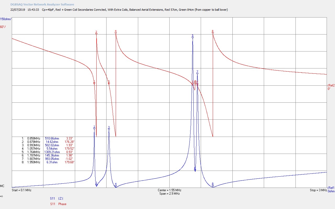
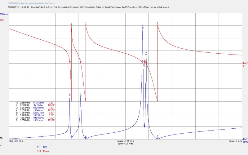
Fig 3.4. Here the lengths of the extra coil extensions have been adjusted to balance |Z| at M₁ and M₃ at ~500Ω. The RTC extended length was 57cm, and the GRC extended length was 84cm, measured from the copper to aerial join, and to the base of the ball top load. With very fine adjustment, which is very difficult to accomplish, it may be possible to also balance |Z| for the extra coils at M₅ and M₇. This would result in the ideal balanced and equilibrium state, where the electric and magnetic fields of induction are balanced across the entire system, energy storage is equal, the null point is equidistant between the RTC and the GRC, and maximum power can be transferred between the two coils. In practice, when |Z| for the fundamental secondary resonance is equal, as shown, the overall system can be considered to be well-balanced, and will perform close to its maximum performance. Very slight adjustments to the drive frequency from the generator can then be used to nudge the system into the best overall balance and match. F_S at M₁ is now 858kc/s which is now close to the original drive frequency of the LAG at 848kc/s.

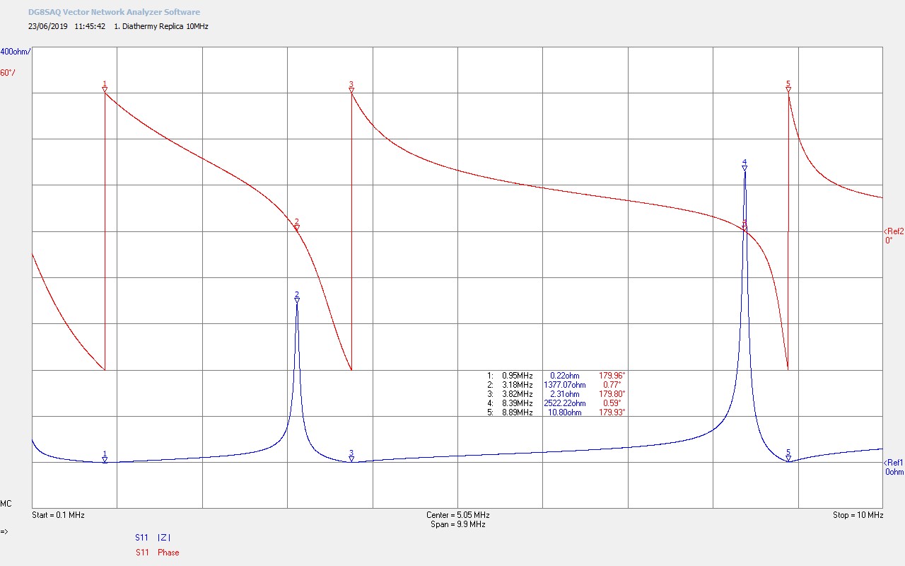
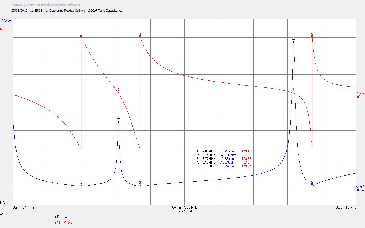
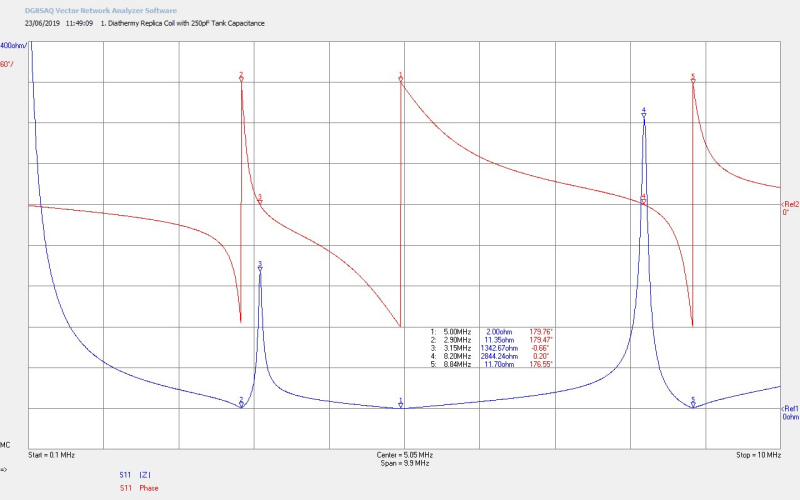
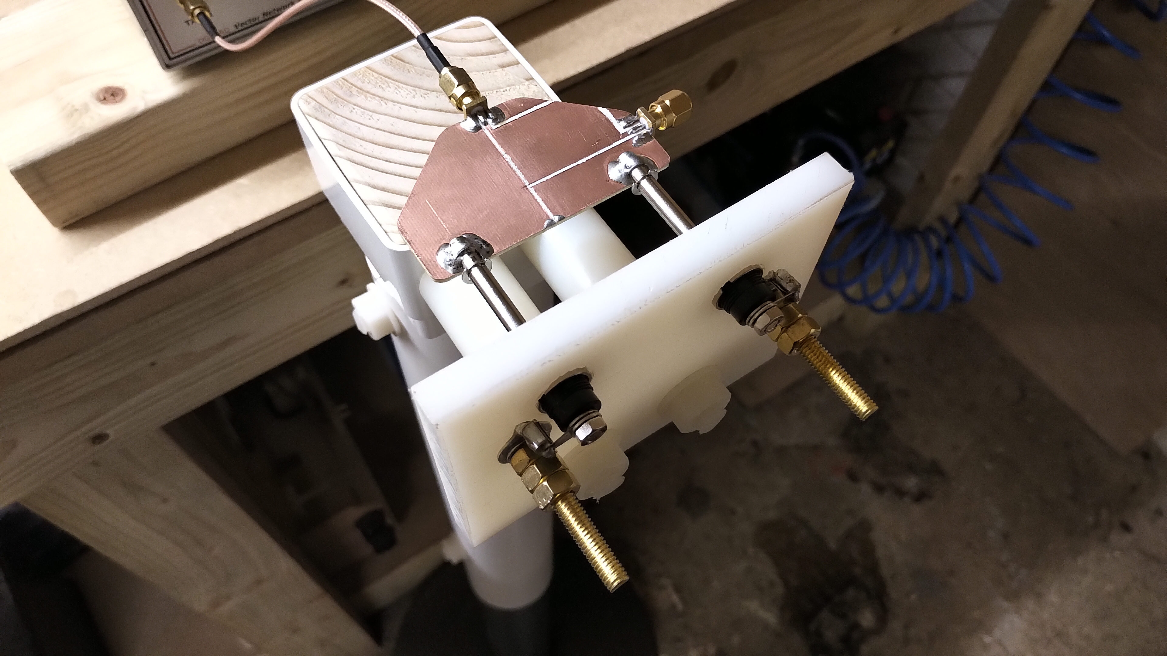
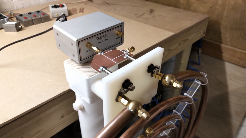
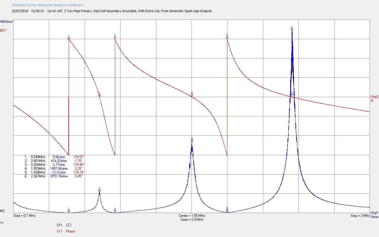
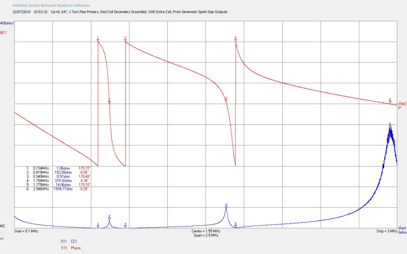
Fig 3.5. Shows the impedance characteristics of the RTC from the perspective of the SGG. The vector network analyser (VNA) is connected to the outputs of the spark gaps in the generator, so the characteristics include the tank capacitance of 6.1nF and the primary coil, which in this case is 2 turns of 1/4″ copper pipe. It can be seen that the resonant frequency of the primary F_P is somewhat below F_S as M₁ at 549kc/s, and is moving away from M₂ and M₃. F_S has also reduced to 801kc/s at M₂ which also shows that the loading in the primary is too much. The inductance of the primary coil, or the tank capacitance, needs to be reduced in order to establish a better match between the generator and the RTC.

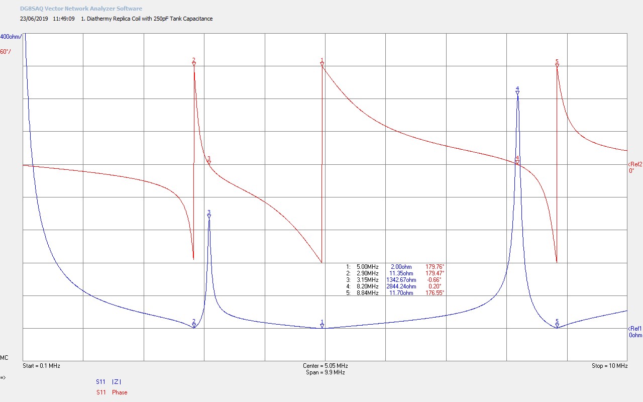
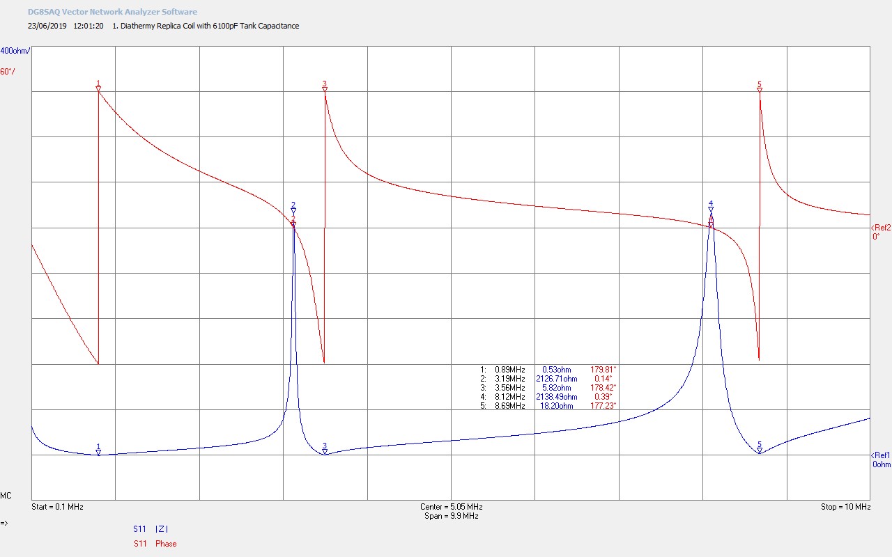
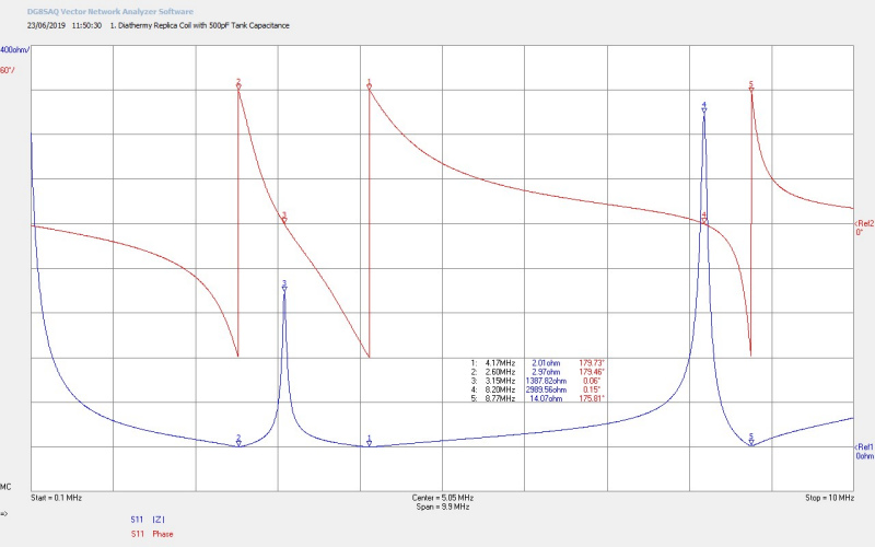
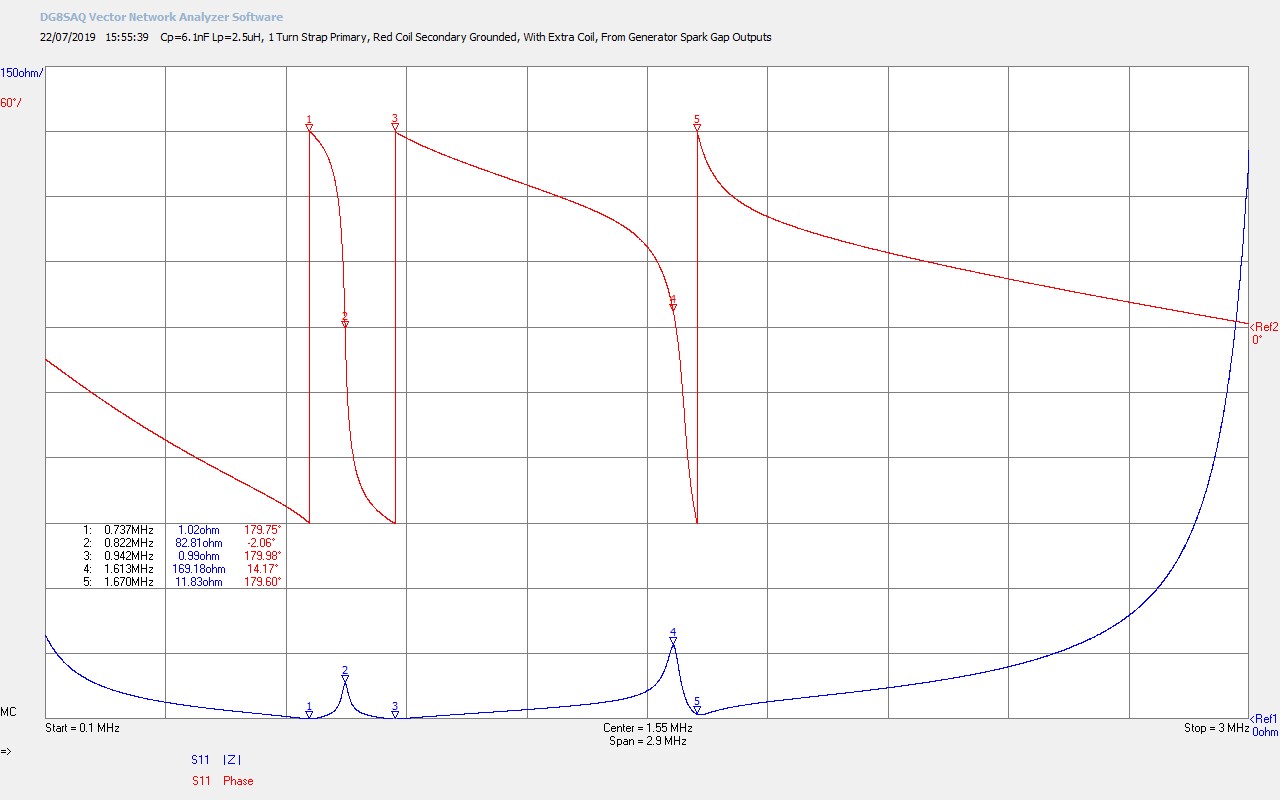
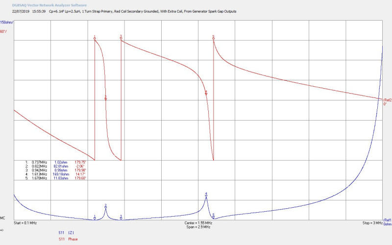
Fig 3.6. Here the number of turns of the primary has been reduced to one, which reduces the inductance in the primary resonant circuit with the generator. M₁ is now closer to M₂ and M₃ and the F_S has now increased to 819kc/s. The tuning between the generator and the RTC has now swung slightly the other way and the primary is pushing upwards on the secondary characteristics. This state is however a better state of tune than that shown in figure 3.5. It can also be seen that F_E for the extra coil is cleaner and less impacted by the primary resonance. Additional fine tuning of the system would ultimately be accomplished by moving one side of the primary connection a certain distance around the circumference of the primary loop, (to form a fractional number of turns in the primary e.g. 1.4), and gain balanced and equidistant spacing for markers M₁ and M₃from M₂.

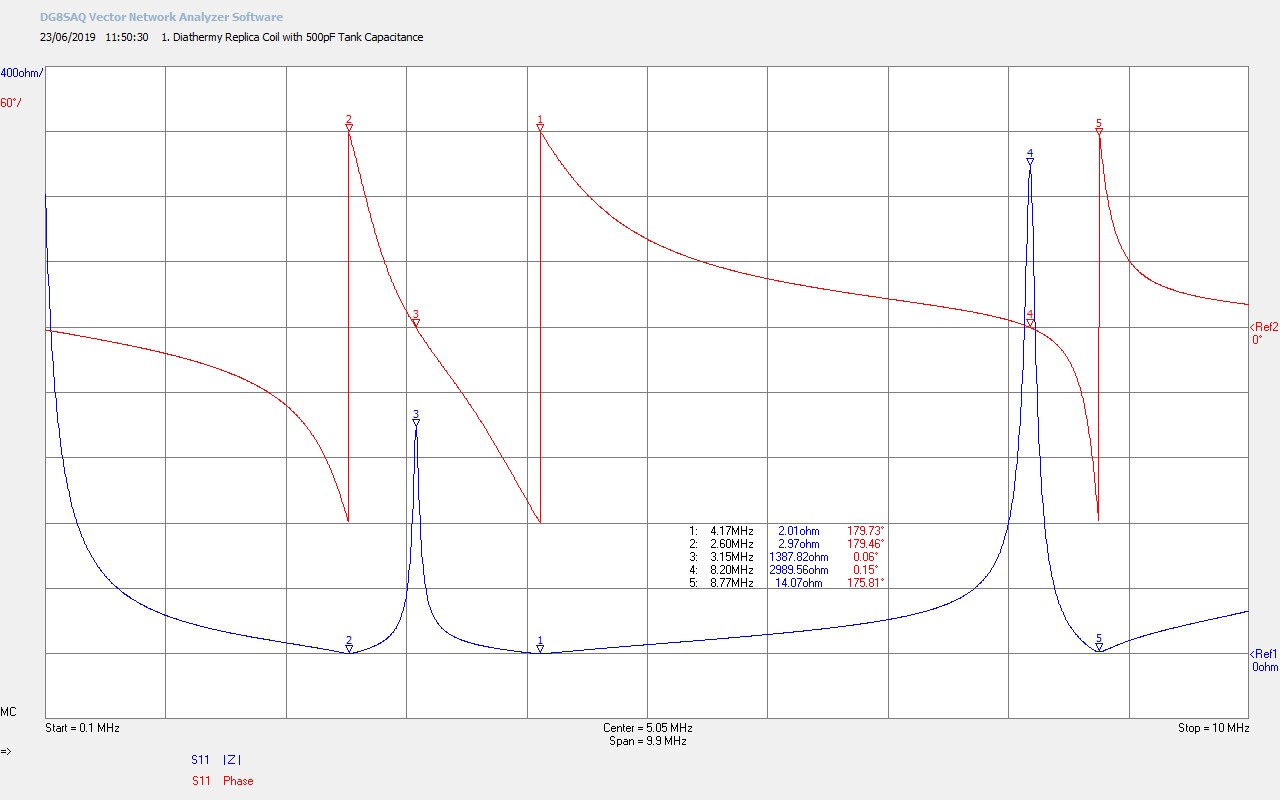
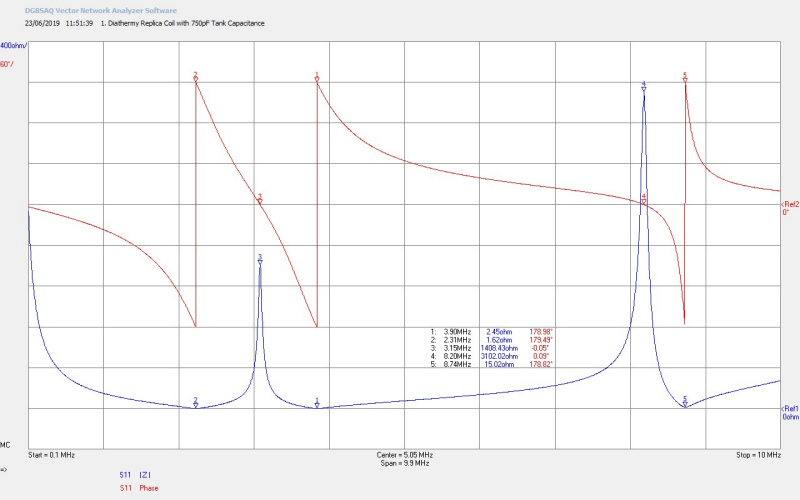
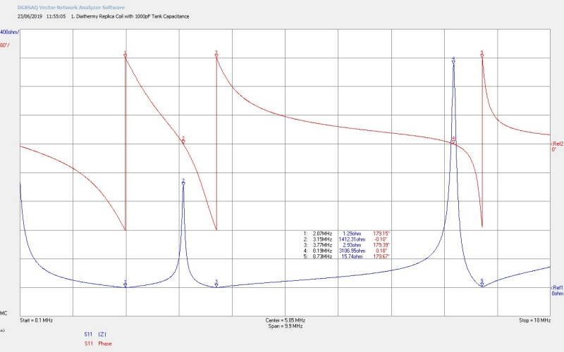
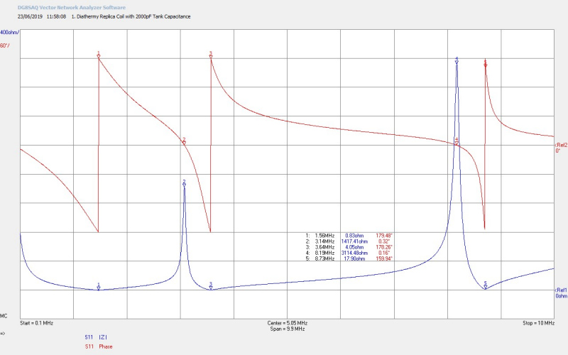
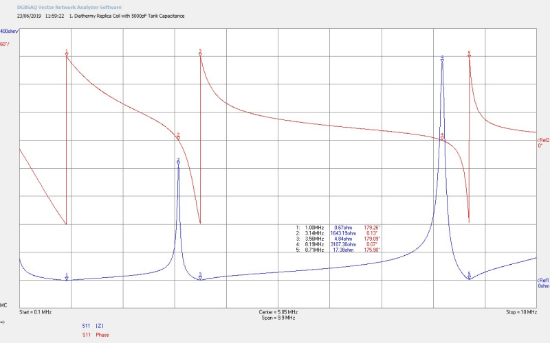
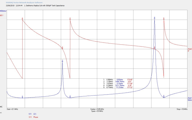
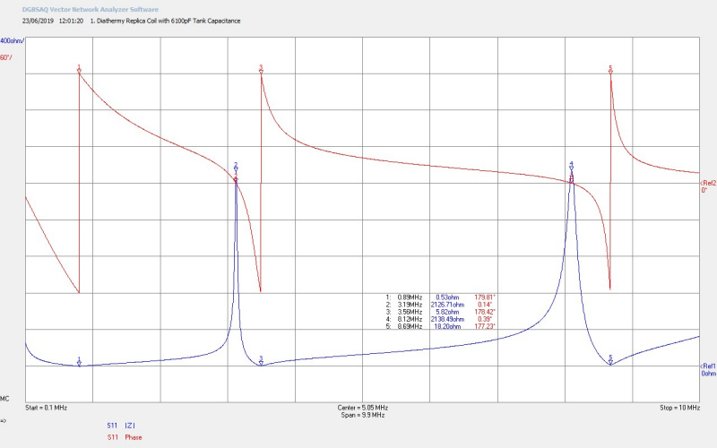
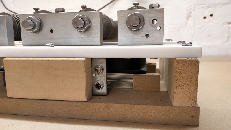
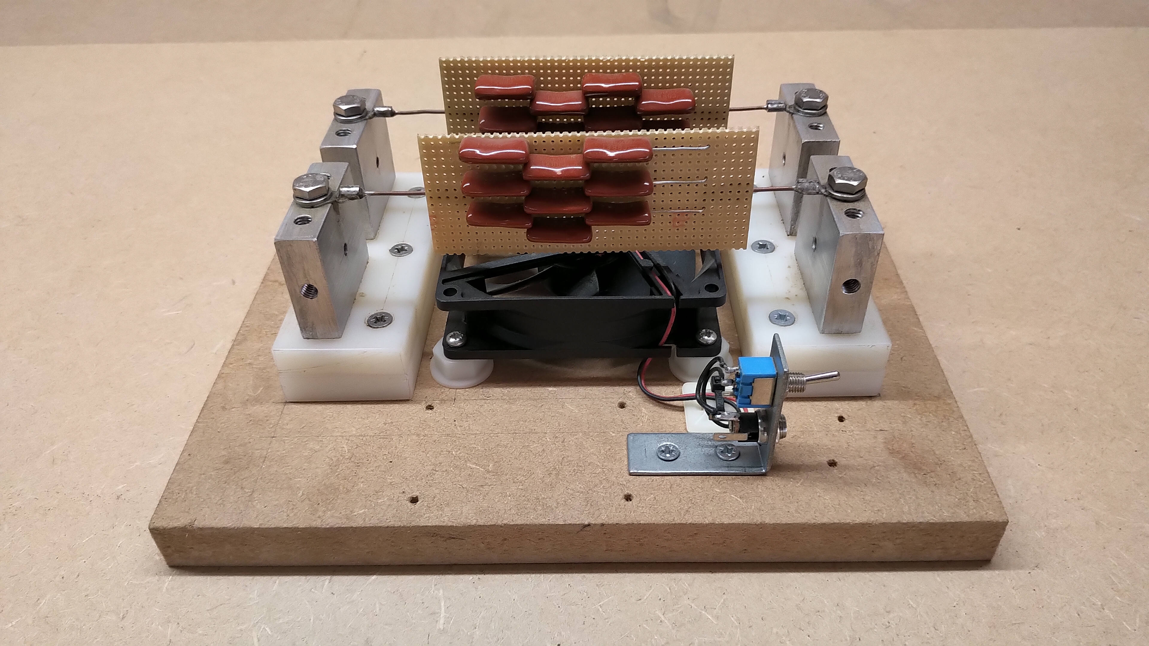
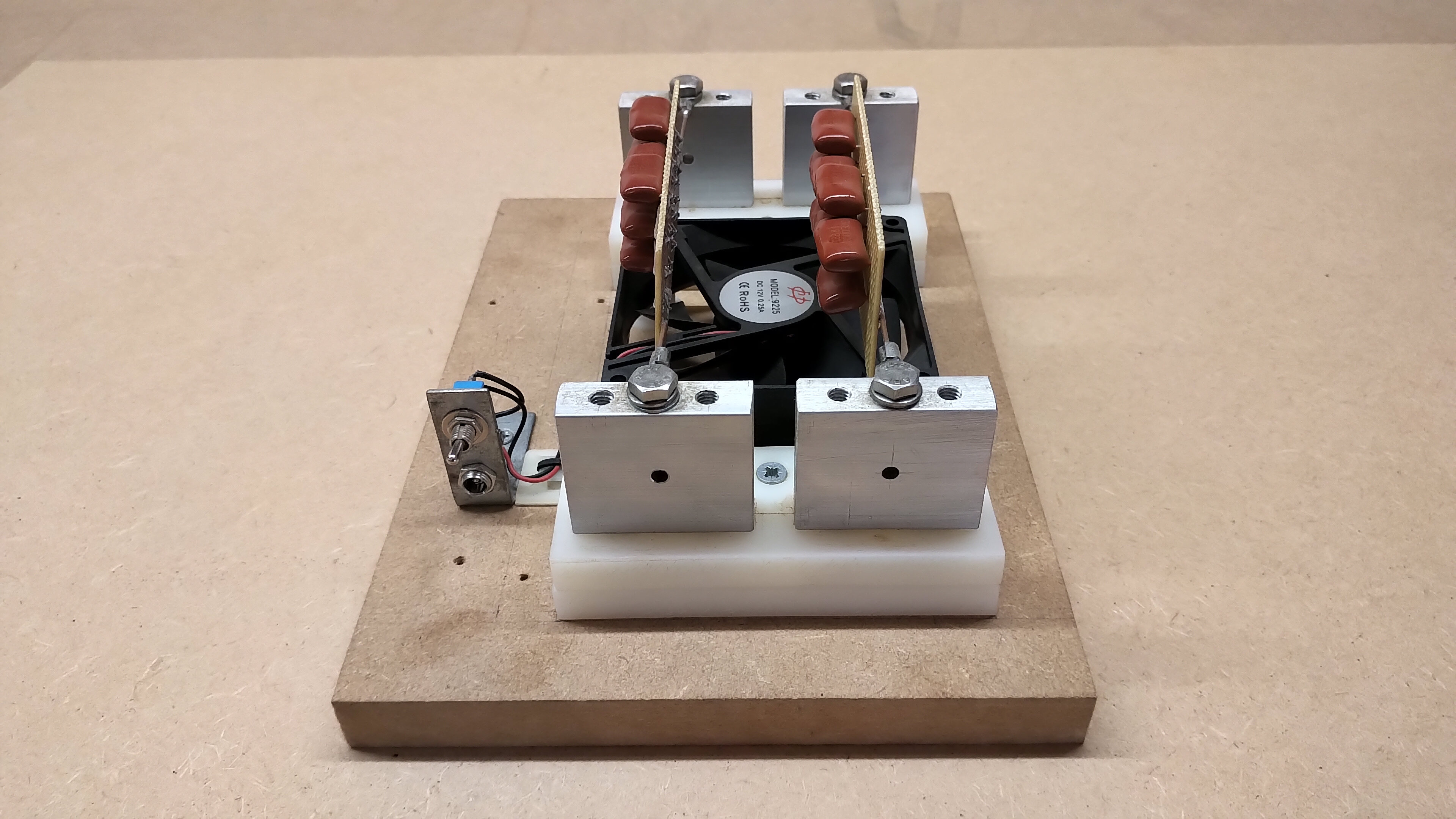
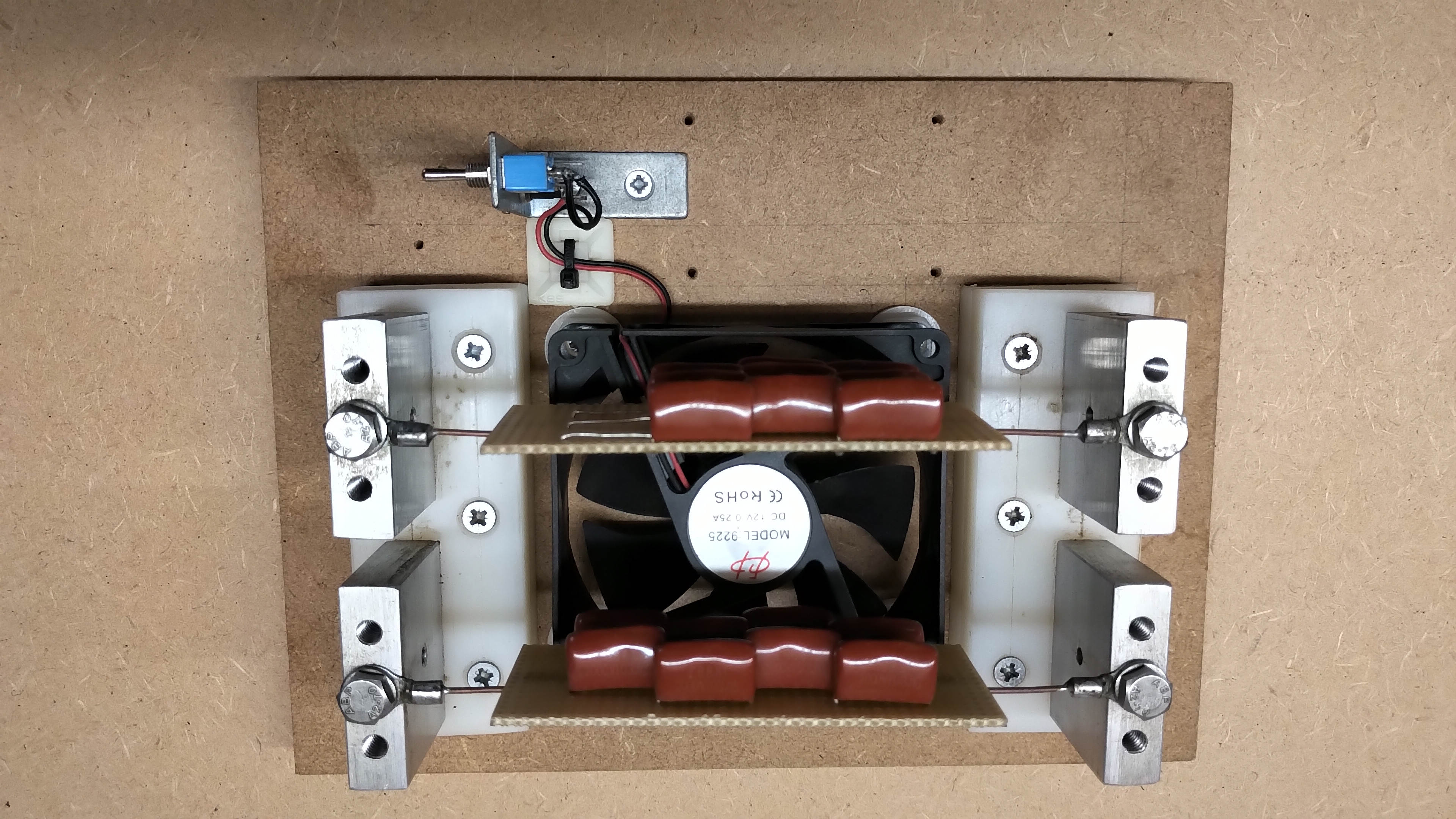
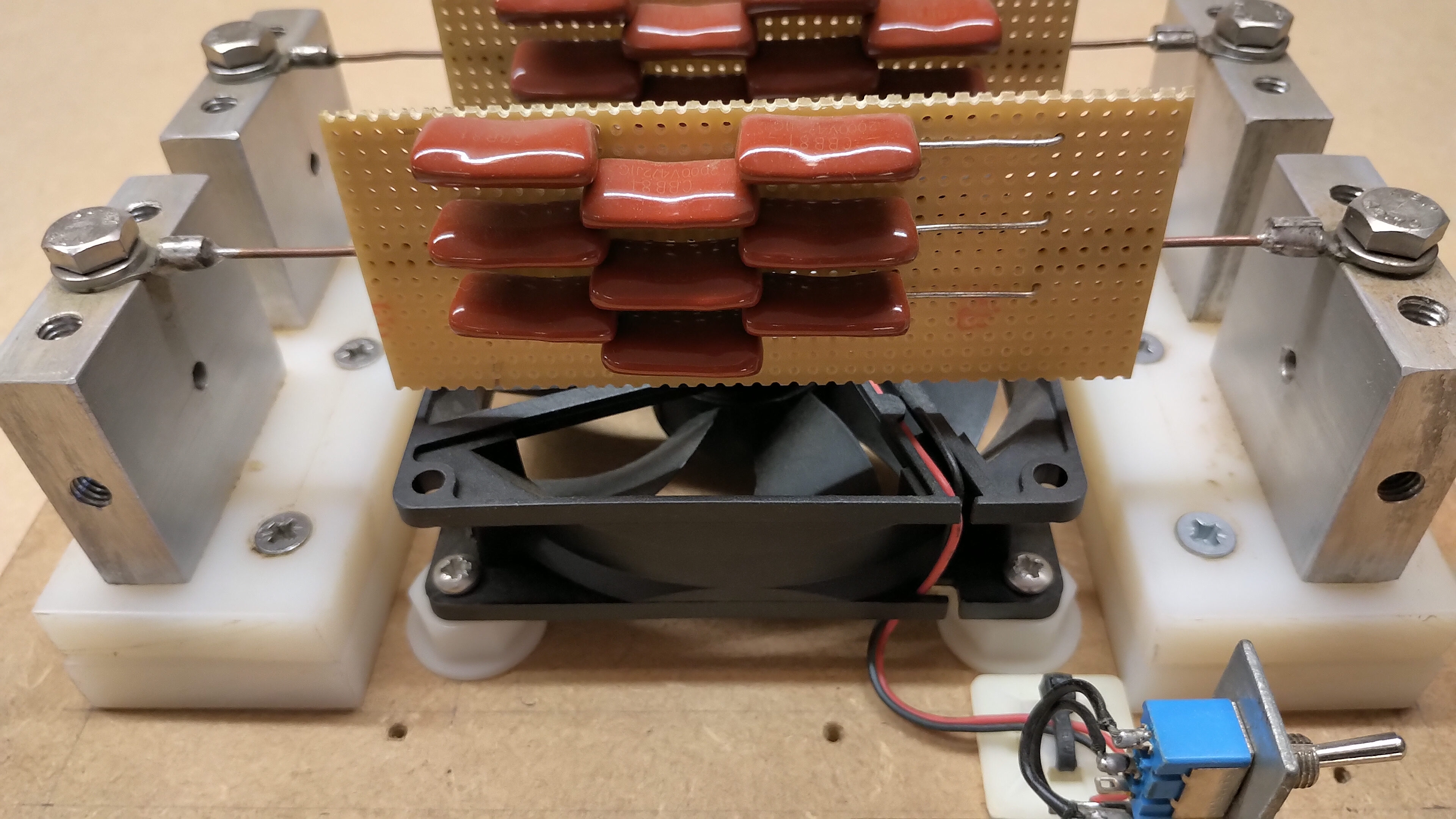
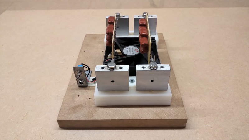
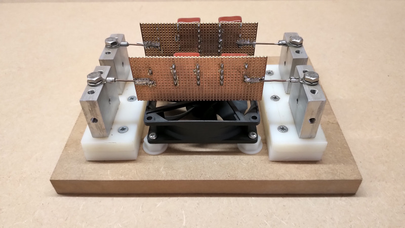
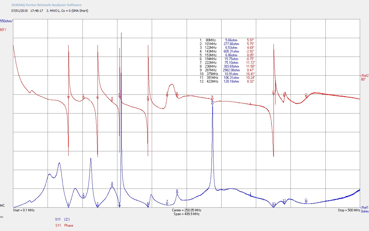
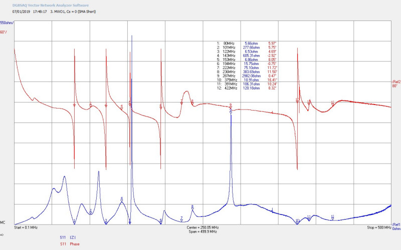
Fig 3.7. Here the single turn copper pipe primary has been replaced with a single turn copper strap, which was deemed to present a lower impedance to the generator, and improve the magnitude of the oscillating currents in the primary. In order to further improve the tuning two 22nF 3kV capacitors in parallel (44nF) were added to one of the outputs of the SGG as shown in the schematic of figure 2.2. This reduced the tank capacitance slightly from 6.1nF to 5.4nF. The inductance of the strap was measured to be 2.5uH which combined with the tank capacitance of 5.4nF provides a theoretical lumped element resonant frequency of 1370kc/s. referring back to figure 3.1 it can be seen that F_S, the resonant frequency of the secondary, without the extra coil at M₁ is 1326kc/s. So the primary circuit tuned and driven at this point has a very close match to the secondary coil, which ensures that maximum energy can be coupled from the primary to the secondary, and then combined with the extra coil, maximum power can be transferred from the generator to the RTC, and ultimately to the GRC when further connected. For the purposes of this endeavour this state of retune was considered adequate for further demonstration and exploration of the Colorado Springs experiment.

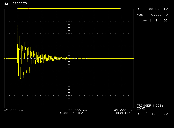
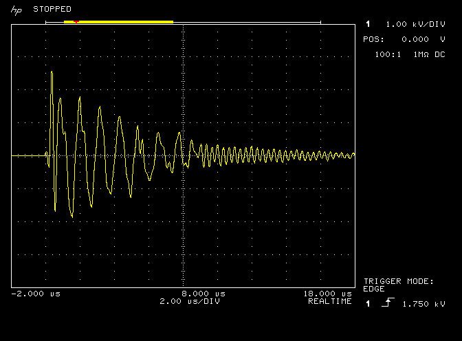
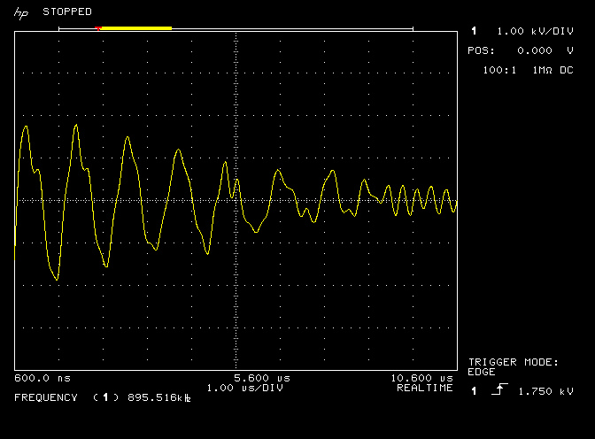
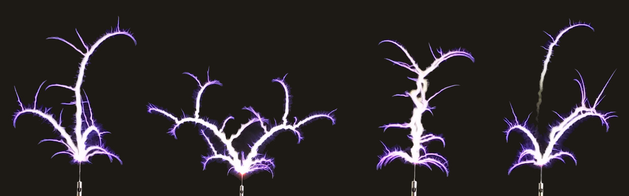
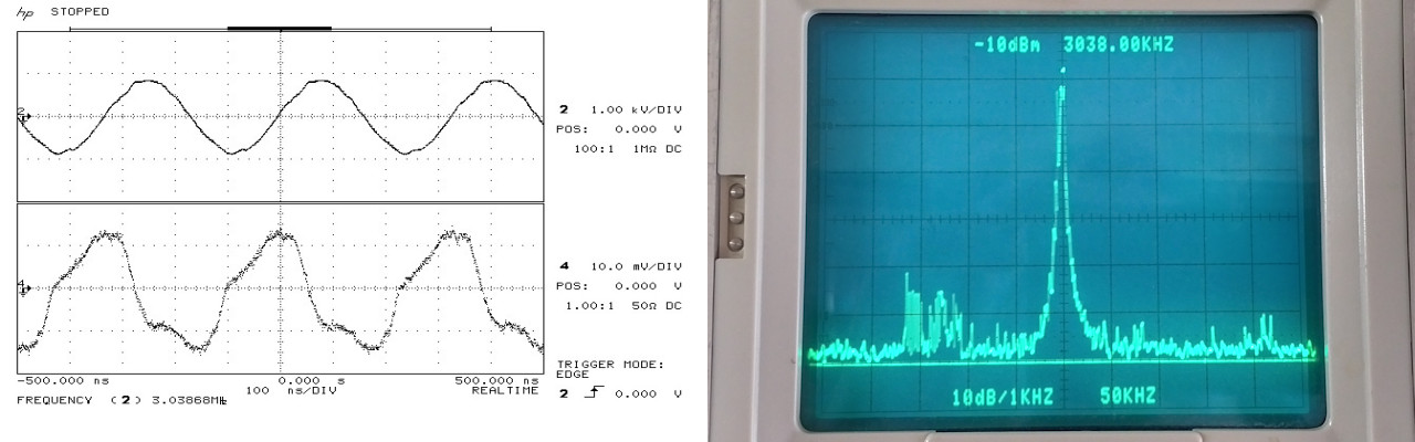
The experimental phenomena observed during the operation of the TCS experiment, retuned to work with the MWO generator, can be seen in the first video on this page.

Summary of the endeavour:

The overall endeavour facilitated the demonstration and exploration of tuning and operating the MWO spark gap generator to work with the Colorado Springs demonstration. In the process the RTC primary and secondary needed to be modified for optimum running with the SGG. Throughout the endeavour a wide range of measurements were demonstrated including:

1. Z₁₁ impedance measurements for the series fed secondary and extra coil, for the RTC.

2. Z₁₁ impedance measurements for the primary combined with the secondary, and the exta coil, for the RTC.

3. Combined Z₁₁ impedance measurements for both the RTC and GRC, where the bottom ends of both secondaries were connected together to form a single wire transmission line.

4. Fine tuning of the system by adjusting the wire length of the extra coil extensions, in order to balance |Z₁₁| in the fundamental and second harmonics.

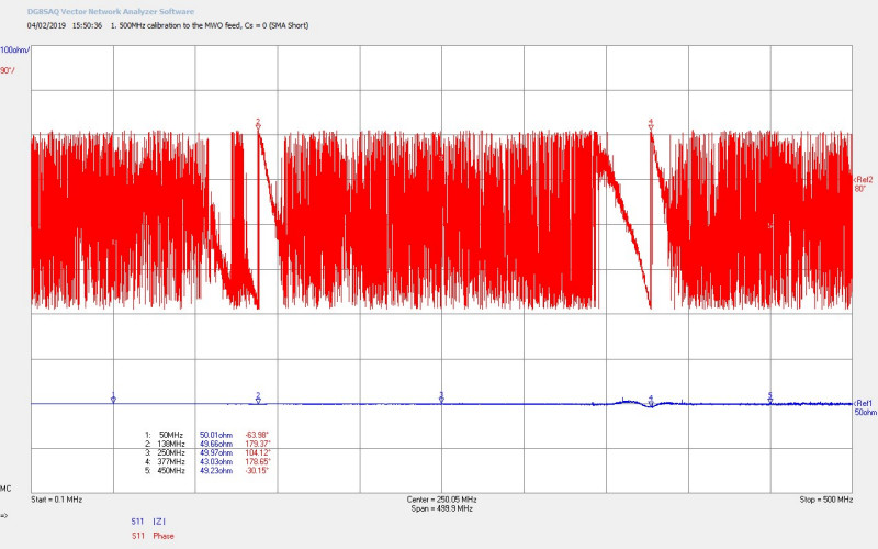
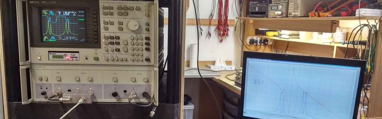
5. Z₁₁ impedance measurements using a computer connected vector network analyser.

The endeavour also facilitated the demonstration and exploration of the following interesting Tesla related phenomena:

6. Single wire electric power transmission.

7. Longitudinal transmission of electric power.

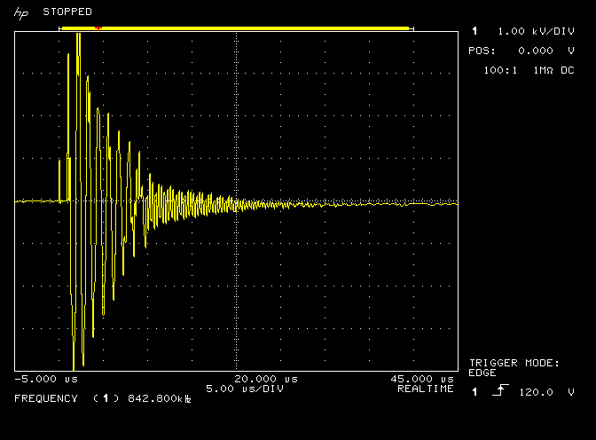
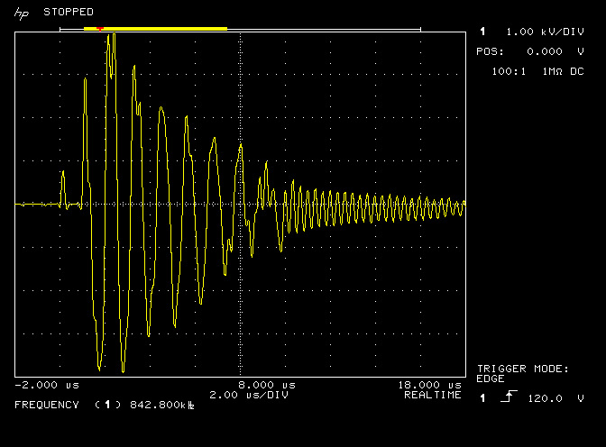
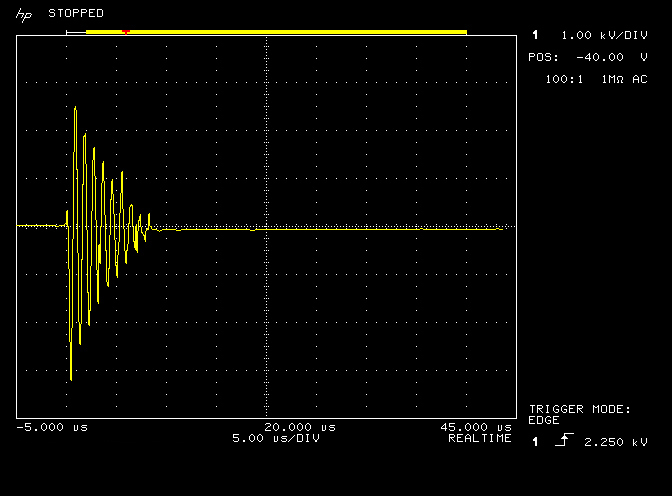
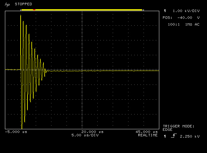
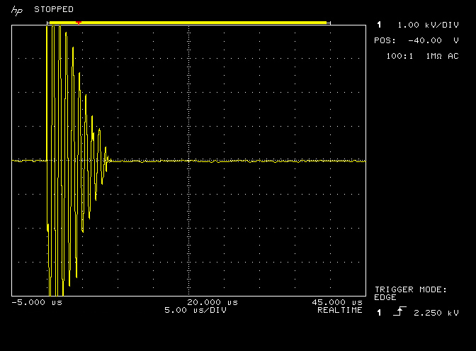
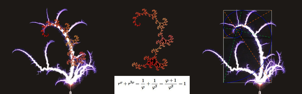
8. Emission of radiant energy pulses from an incandescent bulb.

9. Radiant energy pulses attracting metal to the bulb.

10. Amplification of radiant energy by interaction with a human hand.

11. Transference of electric power between a TMT “transmitter” and “receiver”.

Click here to continue to the next part, ESTC 2022 – Vector Network Analysis & Golden-Ratio/Fractal-Fern Plasma Discharges.

1. ESTC 2019, Energy, Science, and Technology Conference, A & P Electronic Media , 2019, ESTC

2. Dollard E., Preview of Theory, Calculation & Operation of Colorado Springs Tesla Transformer, 2019, EricPDollard

3. A & P Electronic Media, 2019, EMediaPress

4. A & P Electronic Media, AMInnovations by Adrian Marsh, 2019, EMediaPress

5. Vril Science, Lahkovsky Multiwave Oscillator, 2019, Vril

Generators, Spark Gap

Spark Gap Generator Measurements – Part2

30th June 2019

Part 1 of the spark gap generator covered the major components of the system, along with the design steps taken to build a diathermy replica unit (DR). In this part measurements are carried out both in the frequency and time domains, to further understand the operating characteristics, and how best to match the output of the generator to the experimental load. In this part there is also consideration as to how the generator transforms the incoming mains supply to an output suitable for experiments in the displacement and transference of electric power.

The primary purpose of any generator within such an experimental system, arranged to investigate the inner properties and workings of electricity, is to provide the necessary tension to the experiment, in order to change the balance of the electric and magnetic fields of induction within the local region of the experimental system. It is considered that changing the local balance of these fields in turn couples to deeper properties within the energetic dynamics and wheel-work of nature, which according to the purpose or the load of the system generates a response into the local experimental system. In so doing the form of the electrical input to the generator is transformed to another more suitable electrical output under tension. In other words the energetic balance of the system is based on an inter-dependence between the local source, (in this case the generator), and the “need” or purpose generated in the system, (in this case the load). The inter-action between source and load defines the local electrical characteristics of the system under experimentation.

In the case of the spark gap generator tension is established by considerably raising the potential (voltage) of the output, whilst simultaneously transforming incoming alternating currents (ac), to oscillating currents (oc) in both the primary and secondary coils in the DR. In addition, and most importantly for displacement, there is a brief moment before the initiation of the discharge of the spark where the impedance of the space in the gap is low, but no transient discharge has yet started. At this point it is conjectured that displacement occurs, and an impulse current is drawn into the system for a very brief moment before the spark discharge is established.

After this moment of displacement, current starts to flow from the tank circuit through the spark gaps, dissipating the stored energy in the circuit through the normal process of transference, and in so doing generating oscillating currents in the resonant circuits of the primary and secondary. It is conjectured that exploration of these transient impulse currents may indicate a mechanism for additional energy to be injected into the system, and is part of the larger displacement principle being investigated as an inner working of electricity, and originating from the undifferentiated coherent action of the electric and magnetic fields of induction to re-balance the dynamics of the local system.

Figures 2 below show the small signal impedance measurements for Z₁₁ up to 10Mc/s at the output of the spark gaps, (with the HV unit disconnected), and then with progressive change of tank capacitance to show the change in tuning, and the optimum match between the primary and secondary of the diathermy replica (DR) unit:

Fig. 2.1 Input impedance Z11 for the DR over a bandwidth of 10Mc/s, showing the primary resonance at M1, the Tesla secondary fundamental resonant frequency at M2, and the second harmonic at M4.
Fig. 2.2 The primary series resonance M1 has moved to 5.0Mc/s with the tank capacitor reduced to 250pF.
Fig. 2.3 Tank capcitance increased to 500pF shows M1 moving closer to the secondary at 4.17Mc/s.
Fig. 2.4 Theoretical optimum tank capcitance achieved at 750pF where M1 and M2 are equally divided around M3, the primary resonance matches the secondary resonance at 3.15Mc/s.
Fig. 2.5 Empirical optimum tank capacitance reached towards 1000pF as the primary resonance at M1 moves away from M2 at 3.15Mc/s. Discharge in the secondary will cause the secondary resonant frequency to drop towards M1, improving the match between the two.
Fig. 2.6 Primary resonance at M1 falling away from the secondary at M2, reducing the match, and hence the power coupled between the primary and secondary.
Fig. 2.7 Primary resonance M1 moving far away from the secondary reducing the coupled power, limiting the secondary currents, and considerably reducing the strength of the secondary discharge.
Fig. 2.8 Effective tank capacitance that brings the response to the non-adjusted response of the DR, where the series primary resonance M1 is at 0.96Mc/s, and the secondary parallel resonance is at M2 at 3.15Mc/s.
Fig. 2.9 The effective tank capacitance of 6100pF which matches the large signal primary and series resonant frequencies shown in Figures 2.3 and 2.4.

Fig 2.1. Shows the resonant frequencies of the both the primary and the secondary coils in the DR. M₁ (marker 1) is the fundamental resonant frequency F_P of the primary, showing the 180° phase change that takes place at the resonant frequency, and the minimum impedance point of a series resonance where |Z| has no reactive components and only reflects the electrical resistance of the primary coil. F_P at 950kc/s is a result of the series combination of the primary coil inductance and resistance L_P and R_P, and the combined two series banks of tank capacitors C_P, and any stray L and C that result from the inter-connecting wires and boundaries to the surrounding medium. R_P ~ 0.22Ω is low and indicates a good primary coil size and material, which will enable larger discharge currents to flow, facilitating stronger oscillations to be coupled to the secondary, and an improved power transfer between the primary and secondary coils.

M₂ shows the fundamental resonant frequency of the secondary F_S = 3180kc/s, and M₃ the frequency at which a 180° phase change takes place F_Ø180 = 3820kc/s. As is normal for a secondary coil where there is considerable distributed resistance across the coil end points F_S and F_Ø180 do not occur at the same frequency, and the parallel resonance formed between L_S and the distributed capacitance C_S set the fundamental resonance of the coil at M₂. When electrical energy is coupled to the secondary from the primary the coil will resonate at the frequency indicated at M₂.

Where required F_S can be made to more closely match F_Ø180 by adding additional loading capacitance to the open end (top-load) of the secondary coil. This is a very common practice for large discharge Tesla coils, (designed for powerful streamers), where metal toroids are added as a top-load and add additional loading capacitance bringing F_S much closer to F_Ø180. This also reduces the Q of the Tesla coil and hence is not desirable for experimental coils designed to explore the inner workings of electricity.

It should be noted that the fundamental resonant frequencies of the primary F_P and secondary F_S do not correspond at the same frequency, as would normally be expected and tuned for a spark gap driven Tesla coil arrangement. Normally to gain maximum power transfer between the two coils their resonant frequencies will be arranged to be the same through tuning of the primary, (L_p or C_p dependent on the type of coil, how it is constructed, and with what materials). This means that in the DR case less power than optimum is coupled to the secondary, and hence the strength of any discharges from the output of the EHT terminal are reduced. Since the DR is based on the original HGF specifications it is conjectured that this may have been desirable for medical diathermy applications to restrict the strength of the EHT discharges by deliberately mis-matching the resonance of the two coils.

The second harmonic of the secondary F_S2 occurs at M₄ and M₅. If the primary is tuned closer to M₄ then the secondary coil will resonate at F_S2 = 8390kc/s which represents the second odd harmonic of the secondary wire length, 3λ/4. The parallel resonance at M₄ is noted to be quite strong, with a similar Q to the fundamental, indicating that the secondary could have a better response to impulse currents generated in the system. Impulse currents due to there very sharp, high energy, wide frequency band, excite a wide range of resonances within a typical Tesla coil system. The ability for the system to respond to such impulse currents largely depends on the overall Q of the coil’s harmonics. The series resistance at M₅ becomes the limiting factor in how much power can be coupled to harmonics of the coil, and has risen considerably from M₃ from 2.3Ω to 10.8Ω.

It can be noted from part 1 that the designed F^λ/₄ (F_Ø180) was simulated for the coil dimensions, turns, and construction as 3806kc/s which is only ~ 0.4% error from that measured in the small signal Z₁₁ analysis at 3820kc/s, (F^λ/₄ occurs at M₃, and is based on the λ/4 length of the coil when one end of the coil is at a low impedance, and the other at a high impedance).

Fig 2.2. Shows the dramatic effect of reducing the total tank capacitance C_P down to 250pF. The marker number for the primary M₁ has been kept the same despite the order of the coil resonances changing across the 10Mc/s band. M₁ the series resonant frequency of the primary F_P has now moved right up to 5Mc/s, which has also resulted in a reversal of M₂ and M₃ so the that F_S is now above F_Ø180 at 3150kc/s. The effect of moving the primary resonance point, through the tuned primary tank C_P, is to mis-match the primary and secondary resonances the other way, increase the effective series resistance of the primary coil resonance from 0.22Ω to 2.0Ω, but to leave the actual fundamental resonance frequency of the secondary F_S with only a ~1% change from 3180kc/s to 3150kc/s. Increasing M₁ to between the fundamental F_S and the second harmonic F_S2 has also had a more dramatic impact on the frequency of the second harmonic, reducing it from 8390Kc/s to 8200kc/s, a change of ~ 2.3%.

It should be noted that the dependence of F_S and F_Ø180 to tuning in the primary is dramatically different for the flat coil parallel tuned, and the cylindrical case series tuned. For the flat coil, parallel resonance tuned, F_Ø180 remains more constant with changes in C_PP, and is almost exclusively effected only by the secondary wire length, whereas F_S, and its harmonics F_SN, vary very widely based on changes in C_PP. In the cylindrical coil, series resonance tuned, the dependence reverses and F_Ø180 varies very widely with changed in C_PS, whilst F_S, and its harmonics F_SN, remain more constant with changes in C_PS. This emphasises the need for the correct choice in the type of secondary coil used for any specific experiment (e.g. flat, cylinder, equal ratio etc.), and also the correct choice of primary tuning mechanism, (parallel or series). The characteristics and differences, and hence the choice for specific types of experiments, for each of these different coil configurations will be considered and reported in more detail in subsequent posts on the cylindrical coil.

Fig 2.3. Here C_P is now increased to 500pF and M₁ starts to move downwards again towards the secondary F_S. In this case F_P is approaching the point of optimum match where the primary and secondary are equally split between the centre point. With C_P = 500pF the match is still a little high where the primary is resonating at a frequency above the secondary.

Fig 2.4. Here C_P is now increased to 750pF and M₁ and M₂ are now equidistant either side of F_S at M₃. Once again F_S has not really changed significantly and is still at 3150kc/s. This point of match is in principle the most optimum match between the primary and secondary coils, where maximum power can be transferred between the two coils.

In practise and for maximum streamers it is usually preferred to operate this form of cylindrical Tesla coil, where F_Pis slightly below F_S, due to F_S falling when a discharge (streamer) occurs. The discharge causes a change in the impedance of the secondary coil reducing its resonant frequency F_S, bringing F_S during discharge to an optimum match with the primary, allowing maximum power transfer from the tank through to the secondary discharge.

In experiments to explore the displacement and transference of electric power, where it is preferable not to produce discharge streamers (dissipating the energy of the system through transference), the optimum match where F_S = F_P is the preferred condition. This is where the Q of the system is maximum, and the continuity between the electric and magnetic fields of induction between primary and secondary are optimum, which in turn ensures the maximum dynamic stability, and best departure point from a system in equilibrium.

Fig 2.5. Here C_P is now increased to 1000pF, F_Pis slightly below F_S, (observed in the larger gap between M₁ and M₂, than M₂ and M₃), which is around the best empirical match for a Tesla coil designed for maximum discharge as discussed in the previous section.

Fig 2.6. Increasing C_P to 2000pF starts to move F_Pmore rapidly away from F_S, the match between the primary and the secondary is reducing, and hence the coupled energy is also reducing.

Fig 2.7. At C_P = 5000pF F_P is now approaching the DR design of Fig 2.1, F_P= 1000Kc/s, and F_S remains mainly constant at 3140kc/s, only having changed ~ 0.3% as C_P changes in the range 250pF – 5000pF.

Fig 2.8. At C_P = 5500pF F_P is now very similar to the DR design of Fig 2.1, however F_S has not yet increased slightly to match the 3180kc/s in Fig 2.1. C_P is somewhat different to the expected ~ 7200pF of the two Cornell Dubiller tank capacitor banks which in combination is 6 capacitors of 47nF in series.

Fig 2.9. Here C_P has been increased to 6100pF, where F_P matches to the large signal primary resonant frequency observed during the time domain experiments shown below in Fig 3.3 at 895kc/s. F_S which is now 3190kc/s has finally moved slightly away from the previously stable 3150kc/s, but notably is now closer to the DR design of Fig 2.1, and also the large signal secondary resonant frequency of 3214kc/s shown in Fig 3.6 below.

Overall the small signal Z₁₁ analysis of the spark gap generator reveals a wealth of detail in understanding how this generator is characterised in the frequency domain, and how best to match the primary tank capacitance to obtain different operating points according to the purpose of the experimental system.

Figures 3 below show the large signal time domain waveforms of the spark gap generator as measured from the low output tap, and illustrate the different stages of the spark discharge burst both in the primary and secondary coils of the generator. The spark gap generator was being run at an input power of 300W, (monitored using a Yokogawa WT200), which was kept constant throughout the measurement of both Figures 3 and 4. Output waveforms were measured using a Pintek DP-50 high voltage differential probe, (max. 6.5kV up to 50Mc/s), which was connected to a HP 54542C oscilloscope to observe and record the output waveforms.

Fig. 3.1 DR burst discharge and ring-down in the primary and secondary, measured at the primary low (L) output tap.
Fig. 3.2 Time magnified DR burst discharge and ring-down in the primary and secondary, measured at the primary low (L) output tap.
Fig. 3.3 Time magnified DR burst showing the oscillations in the primary coil at a resonant frequency of 895kc/s, and after a phase change the start of the ring-down oscillations in the secondary.
Fig. 3.4 Amplitude magnified DR burst showing the oscillations in the primary and secondary coil, and illustrating the ring-down envelope in the secondary after the spark discharge has finished in the primary.
Fig. 3.5 Delayed and time magnified DR burst showing the last oscillations in the primary and the ring-down of the secondary coil.
Fig. 3.6 Time and amplitude magnified DR burst showing the oscillations of the secondary coil at 3.21Mc/s.

To view the large images in a new window whilst reading the explanations click on the figure numbers below:

Fig 3.1. Shows the burst waveform measured at the low output tap of the DR. The vertical amplitude scale is 1kV/div, and the horizontal timebase is 5µs/div. The oscilloscope was adjusted to acquire the burst in single-shot mode, triggering at a low to high transition of 1.75kV, where the output delay was adjusted to coincide the trigger to the start of the second full horizontal division. The burst waveform is formed of three major sections, where the first is right at the point of triggering and always involves a very sharp impulse type transition, the second a ring-down of specific frequency based on an exponentially decaying oscillation in the primary coil of the DR, and the third, a ring-down of another specific frequency on an exponentially decaying oscillation in the secondary coil of the DR.

The first section occurs right around the moment of initiation of discharge of the spark gap, and includes a very sharp impulse transition, where the amplitude of this impulse can be many times more than the nominal tension of the high voltage supply. This section requires more detailed capture and measurement with a more sophisticated experimental setup, and will therefore be considered and reported in a subsequent post. Here it is sufficient to understand that there is an impulse like start to the spark discharge, which only lasts for a very brief moment around the initiation of the discharge, and produces very narrow and sharp amplitude spikes at the very beginning of the output burst.

The second section is established right after the spark discharge has started, and the energy stored in the two tank capacitor banks is being discharged in the primary circuit. Before the spark discharge is initiated the tank capacitors are charged by line frequency alternating current supplied by the output of the high voltage supply, where the charging circuit is formed by the high voltage transformer connected through the tank capacitors to the primary coil. When the tension across the output of the transformer has risen above the combined breakdown voltage of the spark gap unit, the spark discharge begins and the impedance across the spark gap suddenly changes from an open-circuit to almost a short-circuit.

The inputs to the primary tank capacitors are now shorted together by the spark and the tank capacitors discharge their stored energy rapidly through the primary coil. The resonant primary circuit formed by the tank capacitors in parallel with the primary coil cause the discharge to oscillate at a frequency defined by L_PC_P, and this oscillation lasts until the tank capacitors are completely discharged. How rapidly the capacitors discharge at the resonant frequency and the magnitude of the oscillating currents generated in the primary circuit is dependent on the series resistance presented by the primary circuit, which should ideally be as low as possible, and in the case of the DR was measured in Fig 2.1. to be ~ 0.2Ω.

The oscillating currents in the primary during the spark discharge of the tank capacitors, couple through induction to the secondary of the Tesla coil in the DR, or more clearly, a sudden change to the prior equilibrium state of the electric and magnetic fields of induction energy in the system result in energy being accumulated in the secondary coil. In the third section of the burst discharge this accumulated energy in the secondary transforms to oscillating currents at a frequency defined by the secondary resonant circuit L_SC_S. The secondary oscillating currents decay exponentially in the secondary coil, (assuming no streamer discharge from the secondary), according to the series resistance presented in the secondary circuit. These secondary oscillating currents again couple through imbalance in the electric and magnetic fields of induction back to the primary circuit, where they can be observed in the output waveform as the third section of the ring-down, which dominates the output when the second section oscillations have become sufficiently small.

The complete burst waveform lasts for about 20µs before decaying to less than 1% of its initial amplitude. Bursts are initiated each new cycle of the line frequency, so for UK standard line input at 50Hz to the high voltage supply, a burst is generated every 10ms, (2 per cycle), or at a frequency of 100Hz.

Fig 3.2. Here the horizontal timebase has been reduced to 2µs/div which accordingly magnifies the burst discharge showing more detail in the first, second, and third sections. In the second section and with careful observation it can be seen that the oscillation is not a pure sine wave, it is actually the oscillating currents of the primary circuit with the smaller oscillations of the secondary super-imposed over the top. The super-imposed secondary currents are not easily discernible in the second section because the amplitude of the oscillation in the primary circuit are large.

As these primary oscillations decay away, and after ~ 8µs, a phase change in the output occurs and the secondary oscillations now dominate the output with an envelope that carries the small decaying primary oscillations. In other words the overall burst waveform is a superposition of the oscillating currents in both the primary and the secondary in both sections two and three, where one or the other can be clearly observed based on the energy stored in the respective resonant circuit, and that coupled forward and backward through the inter-action of the two coils.

Fig 3.3. Here the horizontal timebase has been further reduced to 1µs/div and the waveform buffer delay adjusted so that section two dominated with the primary oscillations fills almost the entire trace. The transition to the third section can be seen in the last two divisions of the trace. With section two the main focus of this trace the monitored average frequency of trace 1 can be seen to be 895kc/s which is F_P, the fundamental resonant frequency of the primary circuit. The amplitude of the primary oscillations is almost 4kV_pk-pk at the beginning of the section, and has decayed after 8µs to ~ 1kV_pk-pk.

Fig 3.4. Shows the discharge burst in magnified amplitude against the original horizontal timebase rate. The amplitude has been magnified by a factor of 10 from 1kV/div to 100V/div which illustrates clearly the transition to the third section where oscillations in the secondary coil, coupled back into the primary coil, are a superposition of the both the primary and secondary oscillations, and hence the envelope of the waveform in the third section appears similar to an amplitude modulated waveform. Note: the indicated frequency on this trace is not accurate as it is calculated by averaging together sections 2 and 3, and cannot be considered to be the fundamental frequency of the secondary coil.

Fig 3.5. Here the discharge burst is magnified both in vertical amplitude and in the horizontal timebase, and illustrates more clearly the decay and envelope of the secondary oscillations.

Fig 3.6. Here the discharge burst is further magnified in the horizontal timebase and delayed into the third section of the discharge burst, which shows the monitored average frequency of trace 1 to be 3214kc/s which is F_S, the fundamental resonant frequency of the secondary coil.

The large signal time domain waveforms have also revealed a wealth of detail about the operating characteristics of the spark gap generator, showing the nature and characteristics of the oscillating output waveform, and with well-defined sections that can be corresponded to the frequency domain properties measured in Figures 2. The results have also shown impulse like characteristics in the first section of the waveform, that certainly require more investigation and more detailed measurement to clarify if they relate to, and contribute to, the conjecture of underlying displacement phenomena within electricity.

Figures 4 below show a comparison on the same vertical and horizontal scale of the low, medium, and high output taps. It can be seen that the amplitude of the output increases with each successive tap, consistent with the geometry of the primary/Oudin arrangement of the coils.

Fig. 4.1 DR burst discharge and ring-down in the primary and secondary, measured at the primary low (L) output tap.
Fig. 4.2 Increased amplitude DR burst discharge and ring-down measured at the primary medium (M) output tap.
Fig. 4.3 Maximum DR burst discharge and ring-down measured at the Oudin coil high (H) output tap.
Fig. 4.4 Magnified DR burst discharge and ring-down measured again at the Oudin coil high (H) output tap.

The low tap produces about 4kV_pk-pk initial output, the medium tap 8kV_pk-pk, and the high Oudin tap ~ 11kV_pk-pk but at considerably reduced current. The medium output tap has been determined to be the best tap for driving TMT experiments, and other experimental apparatus suited to the exploration of the displacement and transference of electric power, where there is high output tension combined with stronger oscillating currents.

Summary of the generator results and conclusions so far:

1. The results and measurements for the spark gap generator correspond well between the frequency and time domain, and give a good insight into how this type of generator works, and the type of output that can be generated. The generator presented in parts 1 and 2 were initially used to confirm the experiments and results of Dollard et al.^[1,2], before being applied widely to my own research into the inner workings of electricity.

2. This generator has been proven to be reliable and robust and can sustain indefinitely output powers of 1.5kW, and short bursts over 2kW with the appropriate connections and arranged loads.

3. This generator transforms the low frequency alternating currents of the line input, into high frequency oscillating current outputs, combined with considerably increasing the tension of the output.

4. Analysis, of particularly the time domain results, indicates a first section in the discharge burst that may include impulse currents and effects that are conjectured to involve displacement events. This section requires more detailed measurement and analysis, and will be reported in subsequent posts.

1. Dollard, E. & Lindemann, P. & Brown, T., Tesla’s Longitudinal Electricity, Borderland Sciences Video, 1988.

2. Mackay, M. & Dollard, E., Tesla’s Radiant Matter Replication, 2013, Gestalt Reality

Generators, Spark Gap

Spark Gap Generator – Part1

29th June 2019

In the early days of my research, and before we built the spark gap generator, it was unclear to me which parts of the electrical system were most directly responsible for generating unusual electrical phenomena, whether it be the generator or high voltage source, the types and arrangements of the various coils, or a combination of these elements setup and arranged in a specific manner, tuned in a specific way, and operated in a specific method.

The complete spark gap generator (SGG), including the diathermy replica (DR), and the MMC capacitor bank unit, is shown in Figures 1 below, and mounted on top of, and connected to the high voltage supply:

Fig. 1.1 HV power unit connected to an H.G. Fischer diathermy replica on the top level, with the Tesla/Oudin coils on the left, and the adjustable spark gaps on the right.
Fig. 1.2 Tesla/Oudin coil unit providing EHT output from the Tesla coil, and low, medium, and high outputs from the primary/Oudin coil arrangements. The coils are fan cooled and can run at power levels up to ~1000W continuous, and ~2000W for short bursts.
Fig. 1.3 The tungsten spark gaps can be run in series and parallel arrangements, are fan cooled, and are best driven directly in parallel from the HV unit using two MOTs in series.
Fig. 1.4 Each spark gap is a tungsten electrode pressed into a drilled, fine pitch thread, stainless steel (SS) bolt, with cooling fins made from SS washers. The final static spark unit is particularly robust and can be adjusted to operate at input powers up to ~2500W.
Fig. 1.5 The HV coil unit is wound according to the same parameters and dimensions as an original H.G. Fischer G2 portable unit, and displays very similar operating characteristics.
Fig. 1.6 The coil unit replaced by a cooled, direct capacitor coupled unit, designed to connect directly between the spark gaps and the flat coil tuning unit. Strong, high power, impulses can be supplied using this unit.
Fig. 1.7 The simple arrangment of the spark gaps driving fan cooled capacitor arrays makes for easy generation of high power impulses at double the line frequency 100Hz, (2 x 50Hz UK mains frequency).

Far more consideration is normally given to the experimental components (e.g. coils), their construction, dimensions, materials, and the results that they yield, and much less on the generators that produce the high voltages and currents that are used to power the experimental apparatus.

Over time this appears to have led to an “air of mystery” surrounding the generators that are used in these types of experiments, quite besides a good generator is a complex and involved process to design and build, and can take much more time than any other system component to “get right”. Certainly when I started out by watching the experimental work of Dollard et al.^[1,2], I was very much left with the impression that many of the unusual results obtained were mostly a product of the special generator and components used, and the experimental coils allowed these effects to be transformed, observed, and experimented with.

I have not been alone in these impressions, as I have received very similar comments from others in the field that have not actually built a working experimental system for themselves, but rather still feel that “air of mystery” that surrounds the generator and specialised components and materials in the systems construction. Only by building or contributing to a working experimental system, (including the generator), is it possible to really dispel this “air of mystery”, as it becomes possible to understand and characterise how the generator is producing the types of voltages and currents specific to its type.

In addition to this, many of the components referred to in important works such as Dollard et al.^[1,2,3], may well have been more readily available in the 80s and early 90s, but are now quite scarce, and often command high prices for working items, or “new old stock” components. For example a 1920s H.G.Fischer diathermy machine used as the primary generator in the experiments of [1] are very rare, and when they very occasionally are available, they are expensive. Without understanding what is inside a generator such as this, and how it is working, it is very difficult to know how to build a comparable generator, or whether one will be able to gain the same types of unusual electrical phenomena demonstrated in works such as [1,3].

This was certainly the place I found myself in the early days where I wanted to begin by reproducing and confirming for myself the unusual measurements and results obtained by others, before using this as an established foundation to advance further in exploring my own ideas and insights regarding electricity, and the displacement and transference of electric power. When I started out there were no good examples of a working diathermy machine currently available, (especially in the UK), so I decided to design and build a diathermy replica for myself, and using readily available materials and components. If this generator could be used to explore unusual electrical phenomena then it would certainly for me increase my understanding enormously of how such generators are designed and constructed, whilst also dispelling the “air of mystery”, and providing a generator design that could also easily be used by others in the field. Later I did finally acquire an original 1920s H.G.Fischer diathermy machine and have been able to make a characterisation and comparison between the replica and the original.

The posts reporting the Spark Gap Generator – Parts 1 and 2 are the result of building a working high power diathermy replica, which is now routinely used in my daily experiments, and has contributed significantly in bringing me to a core understanding, that all parts of the electrical system play a specific role in the generation of unusual electrical phenomena. In the exploration into the displacement and transference of electric power each part of the system apparatus must first be measured and characterised carefully to establish a well tuned and balanced overall system, and where the electric and magnetic fields of induction are balanced and in a state of dynamic equilibrium.

From this point it is possible to experiment directly into the properties of electricity, and come to an understanding that the unusual phenomena observed are a product of the inner workings of electricity itself, where the generator and experimental apparatus are necessary to set up the conditions and boundaries required to explore these inner properties. The properties of electricity are there to be revealed rather than “generated”, which also assists greatly in dispelling the “air of mystery” that the generator is the source of the unusual phenomena, but rather, the instrument that provides the necessary tension to trigger the imbalance of the electric and magnetic fields of induction, and hence to observe electrical phenomena within the system. The differences here are subtle but hugely important to the overall understanding of electricity and particularly displacement of electric power.

The circuit diagram for the SGG and peripherals is shown in Figure 2 below, or click here to view the high-resolution version.

Fig. 2.1 Spark gap generator schematic showing the static spark gap, the diathermy replica unit, and the tank capacitor unit.

In the early days in order to replicate the experiments and results of Dollard et al.^[1], it was considered that the diathermy replica (DR) should be as close as possible to the original, which of course posed a challenge when there was no original from which to take measurements, dimensions, construction methods etc. To overcome this a range of references from the internet were studied, along with available circuit diagrams. The most useful references proved to be a combination of material from [3,4,5], and allowed key dimensions and some circuit component values to be extracted from the images and videos.

Click on the following links to view circuit diagrams for various original H.G. Fischer (HGF) diathermy machines, the Model G2, the Model H, the Model CDC, and the Model A^[4].

In any Tesla or resonant coil design it is first necessary to define the desired properties of the secondary coil. With this defined the primary and other components of the system can be designed around the secondary properties. In the case of the DR, and in the absence of any good measurement data, e.g. the resonant frequency of the HGF secondary, the DR secondary was designed according to the known and available dimensions of the HGF secondary, the wire size and type, and the number of turns, (mostly gained from [5]). The dimensions and wire were then adjusted for readily available materials and then key parameters extracted using the software Tccad 2.0^[6]. The DR secondary coil properties were adjusted primarily to match F₀ the primary resonant frequency of the secondary coil, while keeping the physical dimensions as close as possible, whilst using readily available material types and sizes. The original HGF and the designed and adjusted DR properties are shown in the following table:

Original H.G. Fischer Model G Diathermy:

From reference pictures and video^[5]:

Turns: 90

Wire: Solid copper 20 AWG cotton-clad, total diameter 1.0mm

Secondary Former (OD): 2⁵/₈“, 65.7mm

Secondary Coil length: 92mm

Primary Former (OD): 3¹/₂“, 89.6mm

Primary Coil: 6 turns 3/16” copper tube

Oudin extended coil: 11 turns 12 AWG solid (2mm) magnet wire

From Tccad 2.0:

L = 340uH

C = 2.87pF

F₀ = 5066 kc/s

F^λ/₄ = 3978 kc/s

Additional top load C^λ/₄ = 1.78pF

Wire length (W_L) = 18.9m

Diathermy Replica:

Adjusted for available materials to match F₀:

Turns: 98

Wire: 19/32 20 AWG Kynar (PTFE coated), total diameter 1.2mm

Secondary Former (OD): 63mm (standard UK polypropylene pipe)

Secondary Former OD + PTFE_TAPE + PTFE_WIRE = 63.40mm

Secondary Coil length: 120mm (the PTFE wire coating adds additional length)

Primary Former (OD): 90mm (standard UK polypropylene pipe)

Primary Coil: 6 turns 3/16″ annealed copper tube

Oudin extended coil: 11 turns 14 AWG solid (1.6mm) magnet wire

From Tccad 2.0:

L = 350uH

C = 2.84pF

F₀ = 5065 kc/s

F^λ/₄ = 3806 kc/s

Additional top load C^λ/₄ = 2.03pF

Wire length (W_L) = 19.4m

Figures 3 below show how the Tesla/Oudin unit was constructed, and the types of materials used in a simple open structure that can be easily adjusted and modified according to the experimental requirements. Components are mounted on a mdf wooden base, and conductors insulated from the mdf using PTFE and Nylon 66 mounts, bolts, and nuts.

Fig. 3.1 The DR module showing the copper primary coil with extension coil, the output taps to the low, medium, and high outputs, and the secondary coil output connected to a brass ball.
Fig. 3.2 The secondary coil is attached inside the primary plastic tube using nylon locating bolts and a nylon nut as a spacer.
Fig. 3.3 The primary tank capacitors are two series strings of Cornell Dubiller 3kV 47n high voltage capacitors, which are force air cooled when running at high output powers.
Fig. 3.4 The secondary coil is wound using PTFE coated 22AWG silver coated (Kynar) wire, and the output fed to a brass ball mounted on a PTFE insulated mount.
Fig. 3.5 The tank capacitors are mounted on aluminiium supports which in turn are insulated from the wooden base using PTFE/Nylon mounts.
Fig. 3.6 The secondary coil is suspended inside the primary by nylon bolts, and can easily be removed and replaced with different secondary coil's of different specifications.
Fig. 3.7 The secondary coil is wound on a polypropylene pipe coated with PTFE tape to improve the thermal barrier between the pipe and the wire when operating at high output powers.
Fig. 3.8 The primary coil is cooled using a fan mounted beneath the coil, and allows output powers in excess of 1.5kW to be sustained without over-heating the module.

The formers of the primary and secondary coils were first coated with PTFE tape to improve the thermal barrier between the coil and the polypropylene former material when running at high output powers. In addition a small low voltage fan was located under the primary coil to help keep the primary cool at sustained high power outputs. The Tesla EHT output and the HT output taps are all mounted on PTFE insulators both for electrical isolation, but also for good resistance to melting and burning which can occur when drawing discharges from these terminals. Nylon 66 can also be used here, but has lower thermal resistance to discharges, but has the benefit of being a much cheaper material than PTFE.

It is important to note that the secondary coil is located in the primary at the opposite end to the Oudin extended coil. In an early version of the DR the secondary was incorrectly located at the same end as the Oudin extension, which because of the increased tension in both coils easily causes breakdown between the two coils, and led to burn-out of the first secondary coil. The tank capacitor banks are made from 3 series connected Cornell Dubiler 941C03 series 3kV polypropylene film capacitors each of value 47nF, which combined gives 15.7n 9kV for each bank. These tank capacitors have been proven to be long-lasting, and robust, and have never been changed, even with input powers in excess of 1.5kW and even up to 2.2kW for short bursts of power.

The tank capacitors are force air-cooled, and mounted on insulated conductors which allow for easy connection and adaption to the circuit under test. The capacitance of the tank was initially higher at around 47n to match more closely the HGF schematic of the Model A, but was reduced to its current value after the real HGF was acquired and measured. At 47n the available output power was quite a bit less than with 15.7n per tank, as the primary resonance is pushed lower and further away from that of the secondary, hence reducing the primary currents, and hence the power coupled from the primary to the secondary.

Figures 4 below show how the static spark gap (SSG) unit was constructed.

Fig. 4.1 The SSG module showing four static spark gaps connected in series via their aluminium mountings.
Fig. 4.2 The spark gap spacing for each gap can be fine adjusted using the insulated handles, and can be tuned for optimum performance whilst running.
Fig. 4.3 The aluminium mounts are insulated from the wooden base by PTFE blocks. The thread of each spark gap bolt is tensioned by a small nylon insert which is compressed using an M4 machine screw and locking nut.
Fig. 4.4 The four spark gaps are force cooled by two fans positioned directly under the gaps. Force cooling allows the gaps to be run in excess of 1.5kW for sustained experimental periods.
Fig. 4.5 Each gap is made from a tungsten rod pressed into a stainless steel bolt with alternating size stainless washers acting as cooling fins.
Fig. 4.6 The fans are powered by a switched low voltage supply isolated below the high voltage gaps by the PTFE mounts.

The SSG unit was at the time the most difficult unit to build when only a large pillar drill, large vice, and bench sander were available in the workshop for mechanical construction. Each electrode of the spark gap is made from ¹/₄” diameter 99.9% pure tungsten rod 1″ long, (not to be confused with tungsten carbide rods), which were pressed using the vice, into the centre of a drilled A2 stainless steel fine pitch bolt. The bolt had a 6.2mm hole centre drilled, by mounting the bolt in the drill chuck and clamping the drill stationary on the stage, and opposite to how a drill press is normally used. This arrangement made a very rudimentary “lathe” and made it easier to drill a centralised 1.5″ hole down the centre of the bolt. The tungsten electrode was then pressed into the bolt leaving 5mm externally for the spark electrode. Alternating stainless steel washers (large and small) were then threaded onto the bolt and finally tightened with a thin stainless steel nut to form the cooling fins of the electrode body.

Each pair of electrodes were then mounted in threaded aluminium blocks, locked in place with a nut on one side, and with a threaded bakelite handle on the other, to allow adjustment of the spark gap space by winding the bolt in or out of the aluminium block. The aluminium blocks were arranged and mounted to form a series connection of all four spark gaps, and also allowing for tapping from any of the 4 stages for experiments using a single gap, all the way up to 4 series gaps, or 4 parallel gaps with shorting shunts. The adjustable electrode was tensioned in the alumium thread by a small compressed nylon rod, ( from an M3 nylon bolt), which was inserted in a vertical hole drilled above the thread, and then tensioned using a screw locked in the correct place by a nut.

The aluminium spark gap blocks are mounted onto PTFE insulators and then mounted to a wooden base where each gap is suspended above force cooling provided by a pair of low voltage plastic fans mounted into the base of the unit. Overall the SSG unit is robustly constructed and can withstand very large powers in constant use. Tuning of the gaps for optimal running can be made carefully during operation via the four insulated adjustment handles, and is demonstrated in the operation video in Part 2.

Figures 5 below show the MMC tank capacitor bank (TCB) which was used to remove one of the tuned primary stages, and hence increase the efficiency and optimisation of the generator driving, for example, the tuned primary of a TMT (Tesla magnifying transformer).

Fig. 5.1 The tank capacitor unit showing the MMC capacitor banks, each a 4.7n 6000V metal film capacitor.
Fig. 5.2 Insulated aluminium blocks mount the MMC banks over forced air cooling powered by a switched low voltage fan.
Fig. 5.3 With forced air cooling the MMC banks work sustainably up to 500W input power. Larger MMC banks can be used for higher input powers.
Fig. 5.4 The MMC banks are mounted on veroboard, and are arranged in three parallel strings to increase current handling.
Fig. 5.5 The MMC banks are arranged in strings of three series capacitors which gives a total maximum voltage handling of 6kV.

The SGG used with the DR as a generator is most commonly connected with one of the L, M, or H outputs to the primary stage of a tuned TMT, of which the primary stage would typically consist of a coil with a parallel tuning capacitor. In this arrangement the DR, which in itself is already a tuned primary stage, is now connected to another tuned primary stage. Whilst this was useful for preliminary experiments in confirming the key experiments and results of Dollard et al.^[1,2] and keeping the generator as close as possible to an original HGF, it has been shown to be more efficient to eliminate the double tuned primary stage by removing the DR and placing the TCB in its place.

The TCB is simply a standalone capacitor unit exactly the same design as used in the input to the DR. Here the TCB is shown with two pcb MMC banks, but the Cornell Dubilier 941C03 series banks could equally as well be mounted in the same way. Figures 1.6 and 1.7 show how the TCB is connected directly to the SSG, and then in turn the output of the TCB is connected directly to the input of, for example, the tuned primary of a TMT, or some other experiment or load. This creates a resonant drive circuit with the TMT coil in series resonance with the TCB capacitors, and is exactly the same arrangement as internally for the DR, and the HGF. Use of the TCB in replacement for the DR has allowed for an easier and more accurate resonant match between the SSG unit and the TMT load, and with greater power transfer between the two units. Impedance measurements are also simplified by removing one resonant circuit from the generator chain. A very wide range of capacitors can be mounted on the TCB, and for higher power experiments up to 2.5kW output power, force cooling is available via the low voltage fan in the base of the unit.

Overall the spark gap generator whether used with the DR unit or the TCB unit at the output, has proven to be a robust and reliable generator for a wide range of experiments. It has enabled the replication of the key experiments as presented by Dollard et al.^[1,2,3,4], as well as forming a flexible and powerful tuned static spark generator for my own experiments in the displacement and transference of electric power, as well as telluric transmission experiments.

Click here to continue to part 2 of the spark gap generator where the operating characteristics are measured both in frequency and time, as well as a short video to show its general operation and running.

1. Dollard, E. & Lindemann, P. & Brown, T., Tesla’s Longitudinal Electricity, Borderland Sciences Video, 1988.

2. Dollard, E. & Brown, T., Transverse and Longitudinal Electric Waves, Borderland Sciences Video, 1988.

3. Dollard, E. & Mackay, M., Tesla Radiant Energy Experiment, Bedini-Lindemann Conference, June 29-30, 2013.

4. Mackay, M. & Dollard, E., Tesla’s Radiant Matter Replication, 2013, Gestalt Reality

5. Sergey Z., Fischer Diathermy Narrating and Exploring a 1920’s Tesla Coil, May 2014, Youtube

6. Chapman R., Tccad 2.0 for Windows, 2000.

Generators, H.G. Fischer Diathermy

1920s H.G. Fischer Diathermy

10th May 2019

Later in the research, (and after the replica diathermy unit had been designed and built), I was lucky enough to come across a real 1920s H.G. Fischer diathermy unit (HGF), which although being sold untested, and in unknown condition, looked suprisingly good from the pictures. It survived the shipping from the USA to the UK all in one piece, and on closer inspection proved to be in good physical and working condition, including the thermo-ammeter, and the original fuse. The only part missing was the 6V power indicator bulb.

The unit is an early model GP, which is actually a model G in a compact portable cabinet, with a robust carry handle, and metal cabinet corner protectors. Being from the USA the ac line voltage input is specified at 110V 60Hz with a maximum power input of 500W. In the UK this line voltage requires a step-down transformer, a suitable auto-adjusting 1kW transformer was found to be adequate for long-term operation. This post presents detailed pictures, measurements, and an analysis of the HGF as a spark gap generator, and a comparison to the replica diathermy already built and reported in the Spark Gap Generator Part 1 and Part 2.

Figures 1 below show the front-panel of the unit, and in detail, the construction and configuration of the various inner components of the HGF:

Fig. 1.1 A working 1920s H.G. Fischer medical diathermy machine type GP, (type G portable version), showing the power control, the spark gaps, thermo-ammeter, the primary and Oudin taps, and the Tesla secondary coil terminal.
Fig. 1.2 Inside the diathermy machine showing the primary and secondary coils of the high voltage transformer, the tapped power control choke, twin tank capacitors, and the Oudin/Tesla coil.
Fig. 1.3 The input power control choke has multiple taps and resticts the current in the primary according to setting, reducing the output of the secondary, and hence the strength of the impulse discharge at the spark gaps.
Fig. 1.4 The primary coil of the high voltage transformer, made from multiple layers of AWG 14 magnet wire and mounted on a laminated iron core.
Fig. 1.5 The dual secondary coils are made from AWG 20 magnet wire wrapped in many insulated layers. The iron core mounted coils are series connected, and produce a peak unloaded voltage of ~ 9kV. and a loaded maximum output of ~ 6kVpk @ 100mA.
Fig. 1.6 The outputs from the high voltage transformer secondaries are connected to each end of the three series connected spark gaps. The spark gap bank is in turn connected by solid copper flat bar to the inputs of the two tank capacitors.
Fig. 1.7 Each tank capacitor is made from many sandwiched thin copper sheets separated by thin sheet mica insulating layers. The structure is held together by wooden end blocks insulated by two fabric cotton webbed sheets.
Fig. 1.8 The outputs of the tank capacitors are connected again via solid copper flat bar to the 6 turn 3/16" copper tube primary, which is in turn connected to the 11 turn 2mm copper wire Oudin coil extension.
Fig. 1.9 The other side of the Oudin/Tesla coil shows the low, medium, and high output taps from the primary and Oudin extension coil. The output of the Tesla secondary coil (left end) can be seen connected to the HV insulated terminal connector.
Fig. 1.10 Wooden end cap of the coil removed to show the inner secondary of the Tesla coil, and the insulator retaining stud that holds the coil ends in place.
Fig. 1.11 The secondary coil removed from the main structure. The coil is 90 turns of AWG 20 cotton clad magnet wire wound onto a cardboard former, and held in place with a cured resin.
Fig. 1.12 The main primary coil former with the secondary removed, and importantly showing that the secondary coil is to the front-end, overlapping with the primary, but not with the Oudin extended coil.

The actual circuit diagram for the HGF, which was obtained by opening and measuring the unit, is shown in figure 2 below, or click here to view the high-resolution version. Click on the following link to view the original circuit diagram which appears the closest match to this unit model, and comes from the original Model G2.

Fig. 2.1 Schematic showing the H.G. Fischer Model GP medical diathermy unit, as confirmed and measured directly from a working unit.

The line input is connected through a switch, (also with outputs for a foot switch), to the input of a multi-tap choke. The choke is designed to restrict the current, based on the output tap setting, through the primary of the high voltage transformer, and hence control the output voltage of the transformer and the strength of the spark discharge. The model G has 5 power settings which control the input power measured in the range 75 – 440W @ 120V, (line output of the auto-adjust step-down transformer). The choke is constructed from multiple layers of windings using AWG 18 solid magnet wire, wound over thin cardboard layer separators, and coated in a Shellac type resin to hold all the windings together. The core of the choke is made from many thin mild steel laminations and mounted each end to the front panel by wooden spacer blocks.

The output of the tap selector from the choke is connected to the primary of the high voltage transformer. The primary is mounted on thicker mild steel laminated core that is rectangular in shape, with the primary at one end, and the two secondary coils at the other. The primary is wound again like the choke with multiple layers of, cardboard separated, AWG 16 solid magnet wire, held in place with the same resin, and then externally coated with paper tape. The two secondary coils are again made from many cardboard separated layers, with ~25 windings per layer of AWG 22 solid magnet wire, and structurally held together by thin wooden layers compressed by insulating fibre threaded rod, and plastic threaded round nuts.

The combination of the primary and secondary coils on the laminated steel core forms an early transformer arrangement. The efficiency of this type of basic transformer is not as high as would be expected for a typical modern design, constructed with modern materials. Increased losses in the laminated core and materials lead to more power dissipation and heating during running, although the size and bulk of the construction results in a robust transformer, that can be run all day long at maximum power without overheating. This is further evidenced that the transformer is still functioning correctly, and is not far short of 100 years old!

The two high voltage transformers are connected in series, and with the outer ends of the two coils connected to the outer ends of the 3 series connected spark gaps, via coiled cotton-clad stranded wire. The spark gaps appear to be a tungsten tipped centre electrode, clad with a machined copper heat sink fin. The other end of the centre electrode is very fine threaded, and with a bakelite adjustment handle at one end to fine adjust the gap spacing of each electrode pair. The outer ends of the 3 series connected spark gaps are connected both to the output of the secondary coils, and the inputs to the series capacitors, in the first stage of a typical Tesla^[1] “hairpin” arrangement. Further detail regarding the Tesla “hairpin” circuit and its history is given in a summary presented by Kraakman^[2].

The two series tank capacitors, ~15nF each, are constructed from alternating thin copper conducting sheets with thin insulating mica sheets. These are sandwiched together between two cotton webbed sheets, insulating them from the outer wooden blocks that compress the capacitor sheets together. The wooden end blocks are compressed together by insulating fibre threaded rod, and plastic threaded round nuts. In fig. 1.6 it is important to note that on the left hand tank capacitor there is another smaller capacitor formed on the outside of the wooden block. This is the floating ground connection capacitor important for diathermy use when connected to a patient. This capacitor prevents the final outputs of the diathermy unit to accumulate to very high potentials relative to ground, which would present a considerable discharge danger to the patient from their body to ground. It is somewhat disconcerting to imagine that the safety of the patient, when connected to this type of high tension generator, was only really ensured by the two series tank capacitors and the floating ground connection capacitor. Failure of any one of these three capacitors would effectively connect the patient to around 6kV @ 100mA at the input line frequency of 50/60Hz!

The two tank capacitors are connected to each end of the primary coil, which is 6 turns of ³/₁₆” copper tube, and then extended by an 11 turn AWG 12 solid copper wire Oudin coil extension. The low, medium, and high output taps are then derived from the primary and Oudin extension as shown in the schematic diagram of figure 2. The primary and Oudin extension are wound around a 3¹/₂” primary former which appears to be a resin/mica composite material. The primary turns are separated from each other by a cotton woven thread which matches the diameter of the copper tube and wire. Connection between the spark gaps and the tank capacitors, the primary coil, and the output taps, are via ³/₁₆” x ¹/₁₆” solid copper flat bar.

The secondary coil is a 90 turn 20 AWG cotton coated magnet wire on a 2⁵/₈” cardboard former, and the turns retained in place by the same Shellac type resin. The secondary coil is retained in the centre of the primary former by two wooden end caps, themselves compressed together by another insulating fibre threaded rod, with plastic threaded round nuts. The inner end of the secondary is connected to the common connection as shown in the schematic, and the other outer “hot” end of the secondary is fed through the centre of a bakelite stand-off/insulator through the front-panel and to the high tension Tesla terminal, (ball connector with 4mm socket hole). It is important to note that the secondary coil is orientated within the primary former at the opposite end to the Oudin coil extension, which prevents the very high tensions at the top-end of both the primary and secondary from breaking through the primary former forming a spark discharge path between primary and secondary coils.

The primary output taps are connected through a manually positioned thermo-ammeter shunt that shows rf output current on two ranges 0-1A, and 0-4A. The manual shunt can be positioned to remove the meter from the circuit, or to connect it in high and low range positions. The low range is protected by a 1A slow-blow fuse that shunts a 22Ω 50W wire-wound power resistor. When the fuse blows the shunt across the resistor is removed and the meter is protected by the series power resistor. The overall low-side output of the manual meter/shunt circuit, is connected to the indifferent (ground) terminal on the front-side of the diathermy main panel. The measured component parameters combined with their important physical attributes are shown on the schematic in figure 2.

Figures 3 below show the small signal impedance measurements for Z₁₁ up to 10Mc/s at the output of the spark gaps for both the original HGF and the diathermy replica (DR) unit:

Fig. 3.1 Input impedance Z11 for the HGF over a bandwidth of 10Mc/s, showing the primary resonance at M1, the Tesla secondary fundamental resonant frequency at M2, and the second harmonic at M4.
Fig. 3.2 Input impedance Z11 for the DR over a bandwidth of 10Mc/s, showing the primary resonance at M1, the Tesla secondary fundamental resonant frequency at M2, and the second harmonic at M4.

Fig 3.1. Shows the fundamental resonant frequency F_Pat M₁ of the primary circuit, and the fundamental for the Tesla secondary coil F_S at M₂, and its second harmonic F_S2 at M₄. F_Pat 1120kc/s is the series resonant frequency formed by the combination of the two series tank capacitors C_P connected together by the spark discharge, in series with the primary coil inductance L_P. L_PC_P forms a series resonant circuit where the reactance of L_Pand C_P cancel each other out at resonance, leaving only the series resistance of the primary R_P at M₁, which in this case is 0.49Ω.

M₂ shows the fundamental resonant frequency of the secondary F_S = 2900kc/s, and M₃ the frequency at which a 180° phase change takes place F_Ø180 = 3180kc/s. As is normal for a secondary coil where there is considerable distributed resistance across the coil end, points F_S and F_Ø180 do not occur at the same frequency, and the parallel resonance formed between L_S and the distributed capacitance C_S set the fundamental resonance of the coil at M₂. When electrical energy is coupled to the secondary from the primary the coil will resonate at the frequency indicated at M₂. It is also to be noted that the Q of the resonance at M₂ is considerably lower than expected, showing that losses in the secondary coil, materials, and mountings are considerable, where rf energy is being both dissipated in R_S, and leaking out of the circuit formed by L_SC_S through parasitics to the surrounding medium. The low Q of the secondary considerably impacts the energy stored in the system, and will reduce considerably the rf oscillating currents in the secondary, which can be seen in figures 3.

The second harmonic of the secondary F_S2 occurs at M₄ and M₅. If the primary is tuned closer to M₄ then the secondary coil will resonate at F_S2 = 8140kc/s which represents the second odd harmonic of the secondary wire length, 3λ/4. The parallel resonance at M₄ is noted also to be very low Q, and similar in this case to the fundamental. The low Q of the secondary can most likely be attributed to, firstly, the cardboard former of the secondary coil, which over considerable time will have absorbed moisture, and presents a considerable leakage or parasitic resistance to the windings of the secondary coil. Secondly, the windings in themselves are only cotton-clad un-insulated (bare) magnet wire, which also presents a significant leakage path to a moisture impregnated cardboard former. Thirdly, the cardboard former is mounted to the primary via wooden end boards which themselves can absorb moisture, and when combined with moisture in cardboard former of the secondary could also form a significant leakage between the windings of the primary (bare copper) and the secondary coils. It is conjectured that the Q of the secondary when the HGF was new, or much younger, would have been better than now measured, but still due to the nature of the materials used, would still present a much lower Q than that which can be obtained by using plastic formers, and with magnet wire either PTFE coated, or high temperature varnish coated.

Fig 3.2. For comparison the same small signal impedance measurement is shown from the spark gap generator diathermy replica (DR). Due to the slightly different geometric sizes, of the readily available materials used, for the primary and secondary, and the modern equivalent of the tank capacitors, the key resonant frequencies of the primary and secondary are at slightly different points. However the general characteristics of the frequency markers remains very similar on the horizontal scale. The series resistance of the primary circuit at resonance for the DR is less than half that for the HGF, showing that larger primary currents can be generated in the DR providing stronger output currents in the low, medium, and high primary taps.

The big difference between the HGF and DR is in the Q of the secondary coil, which is very much larger, and well-defined, in the case of the DR. This shows the difference largely between the types of materials used to construct the secondary, which in the case of the DR is a plastic polypropylene former, with PTFE coated Kynar secondary windings, insulated from the plastic polypropylene former of the primary, by nylon 66 connecting bolts. All these plastic insulating mediums do not suffer with moisture absorption over time, do not degrade significantly over normal time spans, and present a very high impedance between the primary and secondary coils, which reduces any leakage currents in the secondary to very low values. Hence the Q of the secondary circuit is very sharp and well-defined.

Figures 4 below show the large signal time domain waveforms of the HGF as measured from the indicated output taps, and illustrate the different stages of the spark discharge burst both in the primary and secondary coils of the generator. The HGF was being run at an input power of ~ 300W, (monitored using a Yokogawa WT200), which was kept constant throughout the measurement. Output waveforms were measured using a Pintek DP-50 high voltage differential probe, (max. 6.5kV up to 50Mc/s), which was connected to a HP 54542C oscilloscope to observe and record the output waveforms.

Fig. 4.1 HGF burst discharge and ring-down in the primary, measured at the primary low (L) output tap.
Fig. 4.2 Time magnified HGF burst showing the oscillations in the primary coil at a resonant frequency of 1077kc/s.
Fig. 4.3 Amplitude magnified HGF burst showing the oscillations in the primary and secondary coil, and illustrating the ring-down envelope in the secondary after the spark discharge has finished in the primary.
Fig. 4.4 Time and amplitude magnified HGF burst showing the oscillations of the secondary coil at 2929kc/s.
Fig. 4.5 HGF burst discharge and ring-down in the primary, measured at the primary low (L) output tap.
Fig. 4.6 HGF burst discharge and ring-down in the primary, measured at the primary medium (M) output tap.
Fig. 4.7 HGF burst discharge and ring-down in the primary, measured at the Oudin coil high (H) output tap.

To view the large images in a new window whilst reading the explanations click on the figure numbers below. For a detailed description of the different sections of the spark discharge refer to the analysis of figures 3 and 4 in Part 2 of the Spark Gap Generator post.

Fig 4.1. Shows the burst waveform measured at the low output tap of the HGF. The vertical amplitude scale is 1kV/div, and the horizontal timebase is 5µs/div. This figure shows clearly the second section, a ring-down of specific frequency based on an exponentially decaying oscillation in the primary coil of the HGF. The third section, a ring-down of another specific frequency on an exponentially decaying oscillation in the secondary coil of the HGF is too small to be observed on this vertical scale. The maximum amplitude of the burst is ~ 5kV_pk-pk, and lasts for about 7.5µs before decaying to less than 1% of its initial amplitude.

Fig 4.2. Here the horizontal timebase has been reduced to 500ns/div and the waveform buffer delay adjusted so that section two dominated with the primary oscillations fills the entire trace. The monitored average frequency of trace 1 can be seen to be 1077kc/s which is F_P, the fundamental resonant frequency of the primary circuit, which corresponds well to that measured in the small signal impedance measurements at M₁, of 1120kc/s.

Fig 4.3. Here the vertical amplitude and horizontal timebase have been reduced from fig. 4.1, in order to show the very small third section of discharge burst, that occurs from the secondary ring-down reflected into the primary circuit. The secondary ring-down is barely 100V_pk-pk and reflects the very low Q of the secondary fundamental resonant frequency F_S, as shown in fig. 3.1. Due to the low Q from the high leakage through the materials used, the third section ring-down has a low amplitude and decays away very quickly, only lasting in this case ~ 4µs after the primary ring-down in section 2.

Fig 4.4. Here the third section has been magnified and the monitored average frequency of trace 1 can be seen to be 2929kc/s, which again corresponds well to that measured in the small signal impedance measurements at M₂, of 2900kc/s.

Fig 4.5. The low tap burst, again on the original scales, for amplitude comparison with the following two figures.

Fig 4.6. Shows the burst waveform measured at the medium output tap of the HGF, and on the same scale as before. The inital burst amplitude has increased to ~ 8kV_pk-pk.

Fig 4.7. Shows the burst waveform measured at the high Oudin output tap of the HGF, and on the same scale as before. The inital burst amplitude has increased to almost 12kV_pk-pk.

A comparison of some of the key characteristics of the HGF and the replica diathermy already built and reported in the Spark Gap Generator Part 1 and Part 2, are shown in the following table:

H.G. Fischer Model GP Diathermy:

Primary Coil: 6 turns 3/16″ copper tube

Primary Former (OD): 3¹/₂“, 89.6mm

Oudin extended coil: 11 turns 12 AWG solid (2mm) magnet wire

Seconday Turns: 90 turns, 20 AWG cotton-clad magnet wire

Secondary Former (OD): 2⁵/₈“, 65.7mm

From figures 3. Z₁₁:

F_P @ M₁: 1120kc/s

R_S @ M₁: 0.49Ω

F_S @ M₂: 2900kc/s

F_S2 @ M₄: 8140kc/s

From figures 4 (large signal time domain, LSTD @ 300W):

F_P: 1077kc/s

F_S: 2929kc/s

V_L (pk-pk): 5kV

V_M (pk-pk): 8kV

V_H (pk-pk): 12kV

Diathermy Replica (SGG Parts 1 and 2):

Primary Coil: 6 turns 3/16″ annealed copper tube

Primary Former (OD): 90mm (standard UK polypropylene pipe)

Oudin extended coil: 11 turns 14 AWG solid (1.6mm) magnet wire

Secondary Coil: 98 turns, 19/32 20 AWG Kynar wire (PTFE coated)

Secondary Former (OD): 63mm (standard UK polypropylene pipe)

From figures 2. Z₁₁ (Spark Gap Generator – Part 2):

F_P @ M₁: 950kc/s

R_S @ M₁: 0.22Ω

F_S @ M₂: 3180kc/s

F_S2 @ M₄: 8390kc/s

From figures 3 LSTD @ 300W (Spark Gap Generator – Part 2):

F_P: 895kc/s

F_S: 3214kc/s

V_L (pk-pk): 4kV

V_M (pk-pk): 8kV

V_H (pk-pk): 11kV

In summary, the original H.G. Fischer medical diathermy unit explored in this post is a robust, self-contained, and easy to use generator suitable for some preliminary experiments and replications in the field of Tesla and electricity research, where high tension oscillating currents are required, e.g. with a TMT experiment. The HGF’s lower overall performance, in comparison to the replica diathermy unit, largely results from age related wear and tear, component degrading, and generally lower quality, or less suitable, materials for high voltage applications. Having said this, the HGF is almost 100 years old, and still working more than adequately as a high voltage generator, which is in itself an impressive accomplishment from another time. Without access to an original HGF, it has been shown in other posts, that a good high performance generator with very similar yet improved characteristics, can be constructed using readily available materials at a very affordable cost.

Click here to continue to part 1 of the spark gap generator where the diathermy replica is designed and constructed.

1. Tesla, N., Experiments with alternate currents of very high frequency and their application to methods of artificial illumination, American Institute of Electrical Engineers, Columbia College, N.Y., May 20, 1891.

2. Kraakman, N., A Brief History of the Tesla Hairpin Circuit, December 7, 2017, Waveguide